Spatial Resource Costrained
Project Scheduling
The allocation and sequencing of activity groups to
spatial resources
Master Thesis Applied Mathematics
A.L. Kok
April 18, 2006
Spatial Resource Costrained
Project Scheduling
The allocation and sequencing of activity groups to
spatial resources
Master Thesis Applied Mathematics
A.L. Kok
s0000949
April 18, 2006
Supervisors: Ir. J.J. Paulus Dr. J.L. Hurink
Committee: Dr. J.L. Hurink Ir. J.J. Paulus
Preface
This thesis is the result of the research I have been doing in the last seven months. This research and thesis form the final phase of my study Applied Mathematics at the University of Twente. I really enjoyed the work that I have been doing in these last seven months, and this is one of the reasons that I decided to continue working at the university of Twente as a PHD-student. I would have never accomplished this thesis without the support of several people. I am very grateful for them and I want to thank some of them in particular.
First of all, I would like to thank my supervisors Johann Hurink and Jacob-Jan Paulus. Their knowledge and experience have brought and kept me on track during my research and their critical notes considering my thesis have improved the quality of it. The discussions with them about the progress of my research have been of great value.
Furthermore, I would like to thank the people working at the chair of DMMP. Thanks to them, I always felt a nice and comfortable atmosphere during my work which had a positive influence on the quality of it. Outside the university, my friends and family have always been supporting me with my research, for which I am very grateful.
Abstract
In this paper, we present a new topic in connection with project scheduling. Since a limited work space can form a restriction to project scheduling prob-lems, an efficient usage of these work spaces (or so-called spatial resources) is required to produce good project schedules. The requirement for the re-source units of these spatial rere-sources is in an adjacent manner (we cannot place a product under construction in separate parts of the work space). A spatial resource unit is not required by a single activity, but by a so-called activity group.
The requirement for adjacent resource units not only appears in project scheduling, but also in several other applications. For example, the prob-lem of scheduling check-in desks at an airport. The reserved check-in desks for each single flight have to be adjacent. Another example appears in the berthing problem, where quay space has to be assigned to ships of differ-ent length, which berth during specified time periods. Within warehouse management and the reservation of hotel rooms, resource adjacency is not required but desirable.
The aim of this paper is to derive a solution method which provides an ef-ficient spatial resource usage within project scheduling. This solution method allocates the activity groups to the spatial resources and schedules the ac-tivity groups, such that good solution possibilities for the overall project scheduling problem are provided.
Contents
Preface i
Abstract ii
Contents iii
1 Introduction 1
2 Problemdescription 3
2.1 Introduction . . . 3
2.2 Existing solution methods . . . 4
2.2.1 Solution methods for the RCPSP and TCPSP . . . 4
2.2.2 The Two-dimensional Strip Packing Problem . . . 6
2.2.3 The Two-Dimensional Bin Packing Problem . . . 7
2.2.4 The Simple Assembly Line Balancing Problem (SALBP) 8 2.3 Objectives of this paper . . . 8
3 Model 10 3.1 Introduction . . . 10
3.2 The TCPS problem with spatial resources . . . 10
3.3 The group scheduling problem . . . 12
3.4 Modeling of two-dimensional spatial resources . . . 17
4 Relation between TCPSP and GSP 19 4.1 Introduction . . . 19
4.2 Extracting the input from the TCPSP . . . 19
4.2.1 Parameters TCPSP . . . 19
4.2.2 Earliest and latest start and completion times . . . 20
4.2.3 Minimum group duration . . . 22
4.2.4 Precedence relations between different groups . . . 26
4.3 The solution of the group scheduling problem translated back to the TCPSP . . . 27
4.4 Objective functions for the group scheduling model . . . 28
4.4.1 Maximizing the idle times . . . 29
4.4.2 Weighed duration . . . 33
4.4.3 Conclusions . . . 35
4.5 Two-phase solution method . . . 35
4.5.1 Introduction . . . 35
4.5.2 Phase one: group allocation . . . 36
5 Solution method 42
5.1 Complexity . . . 42
5.2 Input size . . . 44
5.3 Better modeling to decrease input size . . . 44
6 Computational results 48 6.1 Introduction . . . 48
6.2 Different time horizons . . . 50
6.3 Different scalings of resource capacity and request . . . 51
6.4 Different scalings of release and due dates . . . 53
6.5 Subproblems of GSP . . . 55
6.6 Conclusions . . . 56
7 Conclusions and Recommendations 58 References 60 Appendices 64 Appendix 1: ILP-formulation of GSP . . . 64
1
Introduction
For many companies, project scheduling problems are a big issue. Since companies have a limited amount of resources (machines, manhours, etc.), it is very important to use these resources efficiently. The higher this effi-ciency, the more projects the companies can handle and the more profit they can make. A high efficiency of the resource usage can only be reached by developing good schedules for the activities that have to be executed.
A special type of resources which companies have to deal with, are spatial resources. Spatial resources are the work spaces, where the activities have to be executed. For example, a dry dock is a spatial resource for a company that builds ships. A special property of these spatial resources, is that the requirement for its resource units, is in an adjacent manner. If we, for exam-ple, want to place a ship in a dock, we have to reserve a number of adjacent resource units for it. The adjacency constraint ensures us, that we do not have to break the ship into several pieces to be able to dock it.
The requirement for adjacent resource units not only appears in project scheduling, but also in several other applications. An example is the schedul-ing of check-in desks at the airport. Dependschedul-ing on the number of passengers and the duration of the check-in period, a number of check-in desks is re-quired for each flight, during a certain time period before departure of the flight. The reserved check-in desks for a certain flight have to be adjacent.
Also in the berthing problem, resource adjacency appears. The berthing problem is the problem of finding an assignment of quay space, when ships of different length berth during specified time periods.
There are also applications in which resource adjacency is not required, but desirable. This happens, for example, within warehouse management and hotel reservations. When a customer wants to hire a number of positions in the warehouse during a certain period, then for convenience and cost-efficiency reasons, it is desirable that these positions are adjacent. Within the reservation of hotel rooms, if a number of guests belonging to a group wants to stay in the hotel, then they might desire adjacent hotel rooms.
In this paper, we present a solution method, that tries to deal with the spatial resource constraints to the project scheduling problem in an efficient way. This solution method not only determines an allocation for the activities to the required spatial resources, where resource adjacency is satisfied, but also determines a sequencing of the activities, that get allocated to the same spatial resource units. The solution method tries to find an allocation and sequencing on the spatial resources that provides good solution possibilities for the remainder of the project scheduling problem.
2
Problemdescription
2.1
Introduction
In many practical instances of the project scheduling problem, a limited work space forms a restriction on the problem. This restriction can have a large influence on the feasibility of project schedules. Therefore, it is very important to use the available space in an efficient way. Before we discuss the problem of finding an efficient spatial resource usage in more detail, we present two project scheduling problems, known from literature.
A well-known project scheduling problem is the RCPSP (see De Boer [14] and Brucker et al. [8]), the ‘Resource Constraint Project Scheduling Prob-lem’. The RCPSP is called a resource driven project scheduling problem, which states that the resource capacities cannot be exceeded and the objec-tive is a minimization function of the completion times of the activities. The
time drivencounterpart of the RCPSP is the TCPSP (see Guldemond [20]), the ‘Time Constraint Project Scheduling Problem’. In the TCPSP, deadlines for the activities are given, and in order to meet these deadlines, it might be necessary to hire extra capacity for the resources. The objective of the TCPSP is to minimize the total cost of the hired capacity.
In the standard RCPSP and TCPSP, the work that has to be done is modelled as so-called activities. These activities have a certain request for the available resources. Since space can form a restriction to the problem,
spatial resources were introduced by De Boer [14]. Examples are dry docks in ship yards, shop floor space, pallets, etc. The spatial resources differ from the regular resources in two essential ways.
The first difference is that a resource unit from a spatial resource is not required by a single activity, but by a group of activities, called a spatial resource activity group (or just activity group). The spatial resource unit is occupied from the first moment an activity from such a group starts until the last activity in the group finishes. Since the start time and completion time of an activity group can be determined by different activities, the processing time of the activity group is variable.
The second difference is that an activity group requires adjacent spatial resource units (see Duin and van Sluis [17]). The assignment of spatial re-source units to activity groups, represents the allocation of a product under construction to a certain work space. Since a product under construction can-not be broken into several smaller pieces, the spatial resource units, where a single activity group gets allocated to, have to be adjacent.
The problem that the solution method tries to solve, can be formulated as follows: “Where should we allocate the activity groups, and in which order should the activity groups, that get allocated to the same spatial resource units, be performed, in order to provide good solution possibilities for the overall project scheduling problem (RCPSP or TCPSP)?” We call this prob-lem, the ‘Group Scheduling Problem’ (GSP). In the remaining of this section, we discuss a number of existing solution methods for (special cases of) the GSP, and we state the objectives of this paper.
2.2
Existing solution methods
The GSP is a new topic in connection with the project scheduling problem and no solution methods for the GSP can be found in the literature. For project scheduling problems, like the RCPSP, many solution methods exist. However, the solution strategies that are used for the RCPSP and TCPSP, are not applicable to the GSP. In this section, we give a brief overview of the solution methods for the RCPSP and TCPSP, and we explain, why these solution methods are not applicable to the GSP.
Although no solution methods for the GSP can be found in literature, there are some special cases of the GSP, which are equivalent to well-known mathematical problems. For these special cases, many solution methods can be found in literature. In this section, we also discuss these special cases of the GSP and we give a brief overview of existing literature on these problems. The first of these problems that we observe is the: ‘The Two-Dimensional Strip Packing Problem’. This problem is a special case of the GSP, where only one spatial resource is considered. The second special case of the GSP, is the: ‘The Two-Dimensional Bin Packing Problem’. This problem is a special case of the GSP, where more then one spatial resource can be considered. The last special case of the GSP is a generalization of the Bin Packing problem: ‘The Simple Assembly Line Balancing Problem’.
2.2.1 Solution methods for the RCPSP and TCPSP
The solution methods for the RCPSP and TCPSP can be divided into opti-mal procedures and heuristics. The most successful optiopti-mal procedures for the RCPSP at this moment, are based on branch and bound methods. We mention the algorithms proposed by Demeulemeester and Herroelen [15] and by Stinson et al. [37].
consequency, many heuristics have been developed to find good, but not nec-essarily optimal, solutions within reasonable time. For an extensive overview of these heuristics and the optimal procedures, we refer to Davis [13] and Herroelen and Demeulemeester [21]. Guldemond [20] showed how adaptive search can be used to derive good solutions for the TCPSP.
The reason that existing solution methods for the RCPSP and TCPSP are not applicable to the GSP, is that most of these solution methods, are (partially) based on two observations, that do not hold for the GSP.
The first observation concerns the resource-usage of a set of activities. If, for a set of activities, it holds for every resource, that the total requirement of the activities in the set for that resource does not exceed the capacity of that resource, then all the activities in this set can be in progress at the same time period. A similar observation for the GSP holds for a single time unit, but not when we are scheduling over a certain time period. Namely, if we have, in a similar way, a set of activity groups, such that it holds for every spatial resource, that the total requirement of the activity groups in the set for that spatial resource does not exceed the capacity of that spatial resource, then this set of activity groups can get scheduled at the same time unit. However, when we are scheduling over a certain time period, then the adjacency restriction to the the spatial resource units to which an activity group gets allocated to, makes it impossible to say whether this set of activity groups can get scheduled at the same time period or not. If we, for example, have to allocate two groups, which both require 5 spatial resource units, to a spatial resource with capacity 10, then we can only schedule them at the same time period, if the group which gets started first, gets allocated to one end of the spatial resource. If it gets allocated somewhere in the middle of the spatial resource, then there are not enough adjacent spatial resource units left to allocate the other group at the same time period.
to be scheduled at a certain time, when developing partial schedules.
The existing solution methods for the RCPSP and TCPSP, rely on these two observations. Therefore, the solution methods for the RCPSP and TCPSP cannot be used for the GSP and we have to develop new solution methods.
However, there are some special cases of the GSP, which are equivalent to well-known mathematical problems, for which many solution methods have been developed. In the following subsections, we discuss these cases one by one.
2.2.2 The Two-dimensional Strip Packing Problem
The two-dimensional strip packing problem, first proposed by Baker et al.
[2], is defined as follows: Pack a set of rectangles into a strip of width 1, such that the height that is used is minimized. The width of the rectangles is assumed to be smaller or equal to 1, and they cannot be rotated. This problem is equivalent to the following special case of the GSP.
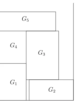
Recall that we consider just one spatial resource. Furthermore, assume that there are no precedence relations between the groups, that each group has a fixed processing time, and that without loss of generality the spatial resource has spatial length 1. Then, if we minimize the latest completion time of the groups, the GSP is equivalent with the strip packing problem. If we namely picture the groups as rectangles where the width represents its spatial length and the height represents its duration, then finding a solution of the GSP is equivalent with placing these rectangles into a strip with width 1 (the length of the spatial resource). Minimizing the height of this strip is equivalent with minimizing the latest completion time of the groups (see also Figure 1).
mathe-G1
G2
G4
G3
G5
Figure 1: Strip Packing
matical models and lower bounds, classical approximation algorithms, recent heuristic and metaheuristic methods, and exact enumerative approaches are discussed.
2.2.3 The Two-Dimensional Bin Packing Problem
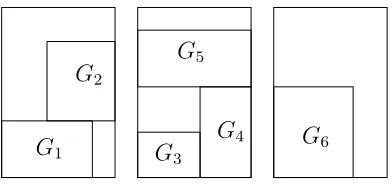
If the GSP has to deal with more then one spatial resource, but the re-sources are identical, then another well-known mathematical problem ap-pears, namely: ‘The Two-Dimensional Bin Packing Problem’, which is de-fined as follows (see Martello et al. [26]): Pack a set of rectangular items in identical rectangular bins, such that the number of bins that is used is minimized. The items cannot be rotated. The two-dimensional bin packing problem is equivalent to the following special case of the GSP.
All spatial resources have equal spatial length, the groups have a fixed duration, there are no precedence relations between the groups, and the groups can be allocated to any of the spatial resources. Given a fixed time horizon, the problem is to schedule all the groups within this time horizon, minimizing the number of used spatial resources.
G1
G2
G5
G4
G3
G6
Figure 2: Bin Packing
The two dimensional bin-packing problem is NP-hard, since already the one dimensional bin-packing problem is NP-hard (see Garey and Johnson [19]). Therefore, several heuristics and approximation algorithms for the bin-packing problem have been developed. Berkey and Wang [5] devel-oped several greedy algorithms for the bin-packing problem. Falkenauer and Delchambre [18], proposed a genetic algorithm. Martello et al. [26] give a survey of recent advances on exact algorithms and effective heuristics and metaheuristics for the two dimensional bin-packing problem.
2.2.4 The Simple Assembly Line Balancing Problem (SALBP)
If we extend the above given special case of the GSP with precedence relations between the groups, then the following well-known mathematical problem appears: ‘The Simple Assembly Line Balancing Problem’. This problem was first proposed by Salveson [35] and is a generalization of the bin packing problem. The SALBP is equivalent with the bin-packing problem where precedence constraints are allowed (see Baybars [4]). Therefore, if we add the possibility of having precedence constraints between the groups to the special case of the GSP, as described in the previous section, then we have a special case of the GSP, which is equivalent with the SALBP.
Since the SALBP is a generalization of the bin packing problem, it is also NP-hard. For an overview of exact algorithms for the SALBP, see Baybars [4]. Bautista et al. [3], proposed a local search heuristic and a genetic algorithm for the SALBP. McMullen and Frazier [28] demonstrated how Simulated Annealing can be used to obtain line balancing solutions when one or more objectives are important.
2.3
Objectives of this paper
develop a solution method, that tries to deal with these spatial restrictions in an efficient way. In order to develop a solution method for the GSP, we first need to derive a model for the GSP. We develop an ILP model, which may form the hose for efficient algorithms. To be able to solve the GSP, we need to know, how we can extract the input for the GSP from the overall project scheduling problem. Furthermore, after solving the GSP, we have to translate the output of the GSP back to the overall project scheduling problem. Therefore, we can formally state the following objectives for this paper:
• Develop an ILP model for the Group Scheduling Problem
• Determine how the input for the GSP can be extracted from the overall project scheduling problem, and how the output of the GSP can be translated back to the overall project scheduling problem.
• Derive a model for the GSP, that gives solutions for the GSP, which lead to good solution possibilities for the overall project scheduling problem.
3
Model
3.1
Introduction
In this section we derive an ILP model for the GSP. Since the GSP results as a subproblem of the project scheduling problem (RCPSP or TCPSP) with spatial resources, we first review the model for the general project schedul-ing problem. Therefore, we review the TCPS-model with spatial resources proposed by Guldemond [20] in the next section. Afterwards, we develop the group scheduling model and an ILP formulation for the GSP. In the last section, we discuss in more detail the modeling of the spatial resources.
3.2
The TCPS problem with spatial resources
For the TCPS problem, activities have to be scheduled before a deadline. These activities can be seen as work that has to be done for some project. If we take, for example, the building of a ship, then all the work that has to be done can be divided into activities, like designing the ship, welding several components of the ship, painting the cabin. We assume that we have
N activities A1, ..., AN. Furthermore, we have a time horizon consisting of
T time units t = 1, ..., T. We assume that every activity Ai has a given
processing time pi, which states that every activity Ai has to be scheduled
for exactly pi time units, and that preemption is not allowed, which states
that if we start on an activity, then we have to keep on working on it without interruption, until it is completed.
Each activityAi also has a release date ri and a due datedi. These dates
bound the time window in which activityAi has to be scheduled. The release
date of an activity depends on, for example, the delivery date of materials that are necessary for performing this activity.
Between some activities, precedence relations exist. A precedence relation between two activities states that one activity cannot start before the other is finished. For example, a ship cannot get painted, before it is constructed. If an activity Aj cannot start before activity Ai is finished, then Ai is called
a predecessor of Aj, and Aj is called a successor of Ai. Sometimes we have
to wait a certain amount of time between the completion of an activity and the start of a successor. This happens, for example, if we have to wait for the paint to dry, before we can do other work on the ship. Therefore we introduce on each precedence relation a nonnegative time-lag lij. This
time-lag lij equals the minimum time difference required, between the completion
time of activity Ai and the start time of activity Aj. With Pi we denote
activity Ai.
To build up a schedule for each activity Ai, we have to determine a
start time SAi, which describes the earliest time bucket at which Ai gets
scheduled. Since preemption is not allowed and we have to process Ai for
exactly pi time units, Ai is completed in time bucket CAi = SAi+pi −1.
Furthermore, activityAi cannot get scheduled before its release date or after
its due date, which implies SAi ≥ri and CAi ≤di. The timelag lij between
activity Aj and its predecessor Ai implies SAj ≥CAi +lij+ 1.
Due to precedence relations, it might be impossible to start an activity at its release date (for example, if activity Ai has ri = 2 and its predecessor
Aj has rj = 1, then Aj cannot start at its release date). Therefore we define
the earliest start time ESAi of an activityAi as the earliest moment in time
when an activity can start, taking into account the timing restrictions of all activities. The latest completion time LCAi of an activity Ai is the latest
moment in time at which an activity has to be completed, taking into account the timing restrictions of all activities. Obviously we have ri ≤ ESAi and
LCAi ≤di. The earliest start time and latest completion time of an activity
define the time window, in which activity Ai can be scheduled.
The earliest completion time ECAi of an activity equals the sum of its
earliest start time and its processing time (ECAi =LSAi+pi−1). The
latest start time LSAi of an activity equals the difference between its latest
completion time and its processing time (LSAi =LCAi−pi+ 1).
For the performance of the activities, a number of resources is required. These resources are, for example, machines and man hours. We assume that there are K resources R1, ..., RK. Resource Rk has a certain capacity Qkt at
time t ∈ {1, ..., T} (the capacity of the resources may vary in time). Each activity Aj requires qjk units of resource Rk during its complete processing.
If, at time t, the total request of all scheduled activities for resource Rk
exceeds its capacity Qkt, then extra capacity can be hired (against a certain
cost). The total cost for hiring this extra capacity is part of the objective of the TCPS problem.
Next to the regular resources, spatial resources appear. These resources are denoted by SR1, ..., SRΛ. The spatial resources are, for example, the
the group finishes. We denote the activity groups by G1, ..., GI. The set of
activities Ai that belong to groupGg is denoted by S(g).
In this paper, we focus on one-dimensional spatial resources, thus, the capacity of the spatial resources is given as a certain length Lλ. This length
can be, for example, the length of a dock. Every activity group Gg has a
certain length requirement lg, which is the request for the spatial resource.
This length can be, for example, the length of a ship that has to lay in a dock. We consider the case that every group Gg has to be allocated to one
specified spatial resource denoted by SRλ(g). Since a ship cannot be broken
into several pieces, the groups require adjacent spatial resource units (see Duin and Van Sluis [17]).
3.3
The group scheduling problem
The group scheduling problem is the relaxation of the TCPS problem, where the capacities of all regular resources (the regular resources are the non-spatial resources) are set to infinity. Using the group scheduling model, we try to find a scheduling of the activity groups, that provides good solution possibilities for the TCPSP.
For the scheduling of the activity groups, two decisions have to be made. First, we have to decide where the activity groups have to be allocated and second, we have to decide for which period the activity groups get scheduled. In order to provide good solution possibilities for the TCPSP, we at least have to ensure that the output of the group scheduling model leaves the room for feasible, or even better, high quality solutions for the TCPSP.
The period that a group occupies a spatial resource is called the duration of the group Dg. This period lasts from the first moment an activity from
such a group starts until the last activity in the group finishes. We denote the start time of groupGg by SGg and the completion time of groupGg byCGg.
Observe that the duration of a group is variable (if for a certain schedule the start and completion time of a groupGg are determined by different activities
and we decrease the start time of the activity that determines the start time of Gg, then the start time of Gg decreases, while the completion time of Gg
remains the same, i.e., the duration of Gg increases). However, as we show
in Section 4.2.3, we can derive a minimum for the group duration, in order to ensure feasibility for the TCPSP.
To restrict the possible values for the start and the completion of the groups, we derive earliest start, latest start, earliest completion and latest completion times for the groups. The earliest start time ESGg of a group
Gg is defined as the earliest moment in time that an activity belonging to
of the activities in Gg. The latest start time LSGg of a group Gg equals
the latest moment in time that Gg can start, such that we can still meet the
time constraints of all the activities. Since the start time of a group equals the earliest start time over the activities in the group, and every activity
Ai in the group has to start before or at its latest start time LCAi to meet
the time constraints, it follows that LSGg equals the minimum over all the
latest start times of the activities in the group. The earliest completion time ECGg of a group Gg equals the earliest moment in time when all the
activities in the group can be completed, which is equal to the maximum over all the earliest completion times of the activities in the group. The latest completion time LCGg equals the maximum over all the latest completion
times of the activities in the group.
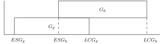
The above considerations only focus on individual groups. However, in general there are also timing relations between the possible processing times of different groups, caused by precedence relations between activities belong-ing to different groups. To ensure that we can fulfill these restrictions after we derived a schedule for the groups, we have to translate these precedence rela-tions somehow into a precedence relation between different groups. There is only one major difference between the precedence relations between different activities and the precedence relations between different groups. A prece-dence relation between two activities implies that the two activities have to be scheduled after each other. For groups however, it might happen that they have to be scheduled at (partially) the same period of time, due to the prece-dence relations between the activities. Assume, for example, that we have two groups G1 and G2 and three activities A1, A2 ∈ S(1) and A3 ∈ S(2).
Furthermore, A1 is a predecessor of A3 and A3 is a predecessor of A2. To
maintain this precedence relations in the TCPSP, we have to schedule the groups G1 and G2 (partially) at the same period of time (at least for the
period that A3 gets scheduled).
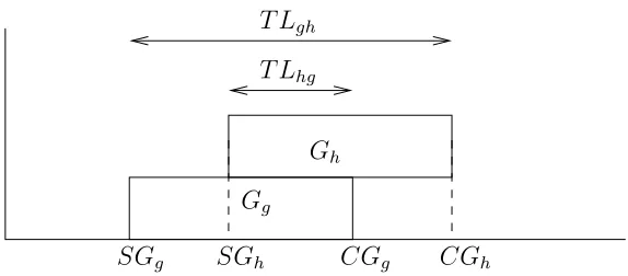
The precedence relation in the TCPSP between two activities implied that the succeeding activity could not start before a nonnegative time-lag was passed after the preceding activity was completed. This kind of precedence relation is not suitable for groups. Therefore we introduce a precedence relation between groups, that states that if group G1 is a predecessor of
group G2, then group G2 cannot complete before a nonnegative time-lag
T L12 is passed, after group G1 has started, i.e. SG1+T L12 ≤ CG2. If we
get back to our example, then we can see that the fact that A1 needs to be
scheduled before A3, implies SG1+T L12≤CG2 and the fact thatA2 needs
to be scheduled after A3 implies SG2+T L21 ≤CG1. Figure 3 clarifies that
these two constraints imply that G1 and G2 will be scheduled at (partially)
SGg SGh CGg CGh
Gg
Gh
T Lhg
T Lgh
Figure 3: Precedence relations between groups
Deriving from all precedence relations between activities of different groups corresponding timelags between the involved groups leads to a set of prece-dence relations between the groups. We denote with Ph the resulting set of
predecessors of group Gh.
To model the GSP, we derive an ILP model. The necessary decisions for the GSP are the start and finish times for the groups and the spatial resource units which are reserved for each group. For the derivation of the start and completion times of the groups, we use the binary variablesgsgtand zgt. The
binary variable gsgt takes value 1 if group Gg starts at time unitt and takes
value 0 elsewhere. The binary variable zgt takes value 1 if group Gg is busy
at time unit t and 0 elsewhere. We can use the following equations to derive the start and completion times of the groups:
SGg =
X
t
gsgt∗t ∀g = 1, ..., I (3.1)
CGg =
X
t
(zgt−zgt+1+gsgt+1)∗t ∀g = 1, ..., I (3.2)
Observe for the first equation that we only addtto the sum whengsgt = 1
and that is exactly when group Gg starts. For the second equation, we have
3 situations:
1. zgt −zgt+1 +gsgt+1 is 0 when group Gg is not busy at time t (zgt =
zgt+1 =gsgt+1= 0 or zgt = 0 andzgt+1 =gsgt+1 = 1)
2. zgt−zgt+1+gsgt+1 is also 0 when group Gg is busy at time t, but also
at time t+ 1 (zgt =zgt+1 = 1 andgsgt+1 = 0)
3. zgt −zgt+1+gsgt+1 is 1 when group Gg is busy at time t, but not at
We see that t only gets added to the sum when t is the last time unit at which Gg is busy. We know that a group Gg cannot start before its
earliest start time and not after its latest start time. The same holds for the completion time which implies the constraints:
zgt =gsgt= 0 ∀g = 1, ..., I, t < ESGg or t > LCGg
CGg ≥ECGg ∀g = 1, ..., I
CGg ≤LCGg ∀g = 1, ..., I
To ensure that every group starts exactly once, we have to add the fol-lowing constraint:
X
t
gsgt = 1 ∀g = 1, ..., I (3.3)
Furthermore, a group can only be busy at time t if it starts at time t or if it was already busy at time t−1, which results in the constraints:
zgt ≤zgt−1+gsgt ∀g = 1, ..., I, t >1 (3.4)
zg1 =gsg1 ∀g = 1, ..., I (3.5)
For the allocation of the groups to the spatial resource units, we use the binary variables bgl and ygl. The variable bgl is set to 1 if l is the first
unit of the spatial resource SRλ(g) to which group Gg is allocated and 0
elsewhere. Since a group Gg may occupy only one ’first’ unit, we have to add
the constraint:
LXλ(g)
l=1
bgl = 1 ∀g = 1, ..., I (3.6)
The variable ygl indicates whether group Gg gets allocated to spatial
resource unit l of SRλ(g). It takes value 1, when group Gg gets allocated to
spatial resource unit l, otherwise it takes value 0. Since the spatial resource units for every groupGg have to be adjacent, groupGg can only get allocated
to spatial resource unit lif it is also allocated to spatial resource unit l−1 or if spatial resource unit lis the lowest index for which groupGg gets allocated
ygl ≤ygl−1+bgl ∀g = 1, ..., I, l >1 (3.7)
yg1 =bg1 ∀g = 1, ..., I (3.8)
We also have to reserve enough space on the spatial resource for every group Gg. We know that group Gg has to be allocated to lg spatial resource
units of its spatial resource. This is satisfied with the following constraint:
Lλ(g) X
l=1
ygl =lg ∀g = 1, ..., I (3.9)
If two groups have to be allocated to the same spatial resource, then we have to make sure that either they do not get allocated to the same spatial resource unit or their scheduling periods do not overlap. To satisfy this, we introduce the binary variable wgh, which takes value 1 if groups Gg and Gh
have at least one common unit in their spatial resource allocation and takes value 0 when the scheduling periods of groups Gg and Gh are not disjunct.
Since wgh cannot take both values 0 and 1, the variable wgh ensures that
at no point in time it cannot happen that two groups are allocated to the same spatial resource unit. The following two constraints guarantee that the variable wgh behaves as described above:
ygl+yhl ≤1 +wgh ∀g 6=h, λ(g) =λ(h), l= 1, ..., Lλ(g) (3.10)
zgt+zht≤1 + (1−wgh) ∀g 6=h, λ(g) =λ(h), t= 1, ..., T (3.11)
The last variable is Dg, the duration of group Gg. The duration follows
simply from the equation:
Dg =CGg−SGg ∀g = 1, ..., I (3.12)
In Section 4.2.3 we derive a minimum for the duration of the group (Dming), which implies the constraint Dg ≥ Dming. In Section 4.2.4 we
derive the time-lag T Lghfor the already mentioned constraintSGg+T Lgh≤
CGh. These two constraints ensure that we can meet the time constraints of
3.4
Modeling of two-dimensional spatial resources
In the group scheduling model, the capacity of the spatial resources is mod-elled as a certain length. This modeling works well for spatial resources like docks, in which ships can only lay in line with each other, but not next to each other. However, there are many applications for which the spatial re-source capacity is not restricted to just one dimension. Examples are, shop floor space, rooms, or pallets. If we consider such spatial resources, then the products can not only be placed in line with each other, but also next to each other (and maybe even on top of each other). In other words, such spatial resources have a capacity in two (or even three) dimensions. In this section, we show how we have to adjust the group scheduling model, such that we can also deal with this these higher dimensional spatial resources.
For two dimensions, every spatial resource SRλ has, next to the length
Lλ, a certain width Wλ. Furthermore, for every group, next to the length
requirement of the group lg, a certain width requirement of the group bg
is given. This modeling is a generalization of the modeling in the previous section, because if we take Wλ = 1 for all spatial resources andbg = 1 for all
groups, then we get spatial resources, where the groups can only be placed in line with each other and not next to each other.
For the allocation of the groups to the spatial resource units, we now use the binary variables blgl, ylgl, bbgb and ybgb. The variable blgl (bbgb) is set to
1 if l (b) is the first length (width) unit of SRλ(g), to which group Gg gets
allocated, and 0 in all other cases. To ensure that group Gg has one ’first’
length (width) unit of SRλ(g), we have to replace (3.6) by:
Lλ(g) X
l=1
blgl = 1 ∀g = 1, ..., I LXλ(g)
b=1
bbgb = 1 ∀g = 1, ..., I
Furthermore, variable ylgl (ybgb) indicates whether group Gg uses the lth
bth spatial length (width) unit, or not. To ensure that the spatial length
ylgl ≤ylgl−1+blgl ∀g = 1, ..., I, l= 2, ..., Lλ(g)
ylg1 =blg1 ∀g = 1, ..., I
ybgb ≤ybgb−1+bbgb ∀g = 1, ..., I, b= 2, ..., Bλ(g)
ybgb =bbg1 ∀g = 1, ..., I
To ensure that every group gets enough space on their spatial resource, we have to replace (3.9) by
Lλ(g) X
l=1
ylgl =lg ∀g = 1, ..., I BXλ(g)
b=1
ybgb =bg ∀g = 1, ..., I
The last two constraints that we have to adjust are (3.10) and (3.11). Two groups have spatial overlap on a spatial resource if they both have a spatial length unit as a spatial width unit in common in their allocation. Therefore we replace the binary variable wgh by wlgh and wbgh, such that
wlgh (wbgh) takes value 1 when groups Gg and Gh get allocated to the same
spatial length (width) unit. To avoid spatial resource conflicts, we have to ensure that when groupGg andGhget scheduled at (partially) the same time
period, then at least one of the two binary variables wlgh and wbgh has to
take value zero. In this case it is clear that it should not happen that group
Gg andGh have spatial overlap and get scheduled at partially the same time
period. This leads to a replacements of (3.10) and (3.11) by:
ylgl+ylhl ≤1 +wlgh ∀g = 1, ..., I, h= 1, ..., I, g 6=h,
λ(g) = λ(h), l= 1, ..., Lλ(g)
ybgb+ybhb≤1 +wbgh ∀g = 1, ..., I, h= 1, ..., I, g 6=h,
λ(g) = λ(h), b= 1, ..., Bλ(g)
zgt+zht ≤1 + (2−wlgh−wbgh) ∀g = 1, ..., I, h= 1, ..., I, g 6=h,
t = 1, ..., T
4
Relation between TCPSP and GSP
4.1
Introduction
The GSP is a relaxation of the TCPSP. Therefore, most of the input for the GSP can be taken directly from the TCPSP. However, to ensure that the TCPSP is still feasible after solving the GSP, we have to add certain restrictions to the GSP, which cannot be taken directly from the TCPSP. In the previous section, we already mentioned that, in order to ensure feasibility of the TCPSP, a minimum for the group duration has to be derived (Section 4.2.3) and in certain cases also precedence relations between different groups (Section 4.2.4).
After we solve the GSP, we have to translate the output of the GSP back to the TCPSP. This translation can be done in different ways. We discuss in Section 4.3 the advantages and disadvantages of the different ways and show how the translation can be done.
The aim of solving the GSP, is to provide good possibilities for getting solutions of the TCPSP. Whether these solution possibilities are provided or not, depends strongly on the objective function used for solving the group scheduling model. Therefore, we discuss in Section 4.4 possible objective functions and make a choice between these possibilities. In Section 4.5, we propose a two-phase solution method for the GSP.
4.2
Extracting the input from the TCPSP
In this section we derive the input for the group scheduling model, that cannot be taken directly from the TCPS-model. The input which we have to derive are the earliest and latest start times of the groups, the earliest and latest completion times of the groups, the minimum duration of the groups, and the precedence relations between the groups with the associated time-lags. Before we derive this input, we summarize the parameters introduced to the TCPS problem in Section 3.2, and we add some new parameters, which are useful for the derivation.
4.2.1 Parameters TCPSP
Ai : Activity i.
S(g) : Set of activities Ai that belong to group Gg.
ri : Release date of activity Ai.
di : Due date of activity Ai.
pi : Duration of activity Ai.
Pi : Set of direct predecessors ofAi.
Si : Set of direct successors of Ai (Si ={Aj|Ai ∈Pj}).
lij : Minimum time-lag between the completion time of activity Ai and
the start time of activity Aj, for Aj ∈Si.
Pi : Set of all predecessors of Ai, i.e., Pi =Pi∪
Pj|Aj ∈Pi .
Si : Set of all successors ofAi Si =
Aj|Ai ∈Pj .
ESAi : Earliest start time of activity Ai.
LSAi : Latest start time of activity Ai.
ECAi : Earliest completion time of activity Ai.
LCAi : Latest completion time of activity Ai.
Asg : Artificial start activity of group Gg (explanation in Section 4.2.3).
Atg : Artificial end activity of group Gg (explanation in Section 4.2.3).
4.2.2 Earliest and latest start and completion times
For the derivation of the earliest and latest start times, and the earliest and latest completion times of the groups, we need to make use of the earliest start times and latest completion times of the activities. Therefore, we first show how to derive these parameters.
As mentioned before, some activities cannot start at their release date or finish at their due date, due to precedence relations and timelags. Therefore, we define the earliest start time of an activity, as the earliest moment in time at which an activity can start, such that the time constraints of all activities can be met, and the resource requirements are relaxed. The latest completion time of an activity is defined as the latest moment in time an activity can finish, such that the time constraints of all activities can be met, and the resource requirements are relaxed. We can derive the earliest start times with a forward recursion through the precedence network.
determined their earliest start time). For an activity Ai ∈ D, its earliest
start time is bounded by its release date ri and by the earliest completion
time plus the time lag for all its direct predecessors Aj (i.e.,ESAj+pj+lij).
Algorithm 1 summarises this process.
Algorithm 1
Initialize:C, D :=∅.
Step 1:D:={Ai|Pi⊆C, Ai ∈/ C}.
Step 2:For every Ai ∈D do ESAi := max
ri,max Aj∈Pi
(ESAj +pj +lji)
.
Step 3:C :=C∪D. If C =∪iAi then stop. Else go to step 1.
We can derive the latest completion times in a similar way by a backward recursion through the precedence network. The sets C and D are defined in a similar way as in Algorithm 1.
Algorithm 2
Initialize:C, D :=∅.
Step 1:D:={Ai|Si ⊆C, Ai ∈/C}.
Step 2:For every Ai ∈D do LCAi := min
di, min Aj∈Si
(LCAj−pj −lij)
.
Step 3:C :=C∪D. If C =∪iAi then stop. Else go to step 1.
The earliest and latest start and completion times of the groups follow from the following equations.
• ESGg = minAi∈S(g)(ESAi).
• LSGg = minAi∈S(g)(LCAi−pi).
• ECGg = maxAi∈S(g)(ESAi+pi).
4.2.3 Minimum group duration
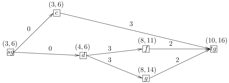
In this section, we derive a minimum on the duration of the groups. This minimum on the group durations is necessary to meet the time constraints of all activities, under the assumption that the regular resources have infinite capacity. As mentioned in Section 3.3, the duration of a group is defined as the period from the first moment an activity within that group starts until the last activity within the group finishes. Since there exist time restrictions on the activities, we can derive a minimum duration for the groups, which is necessary to meet these time restrictions. Before we give a general procedure to derive the minimum group duration, we give a small group example, in which we derive the minimum duration for this group. Afterwards, we show how to derive the minimum group duration in general.
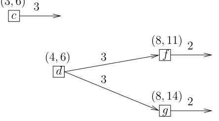
To get a clear view on the problem, we present the example instance in an Activity-On-Node network (AON-network). In this network, the nodes represent the activities, and the arcs the precedence relations. The nodes are labelled with a tuple (ESAi, LSAi), where LSAiis defined as the latest start
time of activity Ai (the latest start time of an activity is simply its latest
completion time LCAi minus its processing timepi). If there is an arc going
from activity Ai to Aj, then Ai is a direct predecessor of Aj. We label the
arcs with the sum of pi (the processing time of Ai) and lij (the time-lag).
If an activity Ai has no direct successor, then we write an outgoing arc at
its node, labelled with its processing time pi. Our example is presented in
Figure 4.
c
(3,6) 3
a
e d
g b
f
4 3 2
3 3
2 (1,3)
(5,8)
(8,11)
(0,2) 2
2
i
(8,14)
(ESAi, LSAi)
pi+lij
(4,6)
G1
In the example, groupG1is given byS(1) ={Ac, Ad, Af, Ag}. This group
is presented in Figure 5. The other activities belong to no group.
d
g f
3 3 (4,6)
(8,11)
(8,14) 2
2 3
(3,6)
c
Figure 5: Activities in group G1, extracted from figure 4
It is easy to see that in this example the minimum duration of group G1
equals 5. This duration can be attained if we start activity Ac and Ad at
time 6, and activity Af and Ag at time 9. On the other hand, the duration
of group G1 cannot be smaller then 5, since the sum of the processing times
of activities Ad and Af, and the time-lag between these two activities equals
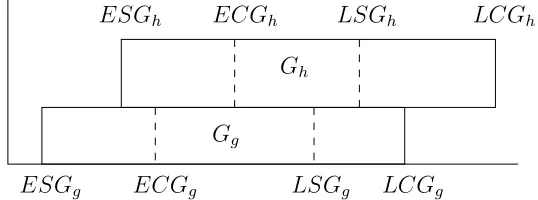
5. Now we show a method to derive the minimum duration in general. To derive the minimum duration of group Gg in general, we first add
two dummy-activities (Asg and Atg) to group Gg, where Asg represents the
start of group Gg and Atg represents the completion of group Gg. We use
these dummy activities, to give a generic algorithm for the derivation of the minimum group duration. We define the processing times of Asg and Atg to
be 0, and we define SAsg :=SGg and SAtg :=CGg. Furthermore, we define
Asg to be a direct predecessor of all the activities in Gg, that do not have
any predecessors within Gg (i.e., Asg ∈ Pi if and only if Pi∩Gg = ∅), and
we define Atg to be a direct successor of all the activities in Gg, that do not
have any successors in Gg (i.e., Atg ∈Si if and only ifSi∩Gg =∅). All the
time-lags for precedence relations in which Asg or Atg are involved are put
to zero. In Figure 6, we see the example group Gg1, where the activities Asg
and Atg are added to the group.
d
g
3 (4,6)
(8,14)
f
(8,11) 3
2
(10,16)
tg sg
(3,6)
0
c
(3,6)
0 3
2
Figure 6: GroupGg1 with dummy-activities Asg and Atg
ESAsg =ESG1 = min
Ai∈S(1)
(ESAi) = 3.
LSAsg =LSG1 = min
Ai∈S(1)
(LSAi) = 6.
ESAtg =ECG1 = max
Ai∈S(1)
(ESAi+pi) = 10.
LSAtg =LCG1 = max
Ai∈S(1)
(LSAi+pi) = 16.
The group duration equals the difference in start times between Asg and
Atg (SAsg = SGg and SAtg = CGg and Dg = CGg − SGg). Finding a
minimum for the group duration, that is necessary to provide feasibility of the TCPSP, is now equivalent with finding the smallest possible difference betweenSAsgandSAtg, such that the time restrictions of all activities within
Gg, can still be met. In the following, we show how to find this smallest
difference.
We first let every activityAi start at its earliest start time: SAi=ESAi.
This gives a feasible schedule (an activity can always start at its earliest start time if all its predecessors start at their earliest start time). Next, we fix the start time of activity Atg at its earliest start time, and we increase the start
times of its predecessors, by a backward recursion through the AON-network, until we reachAsg. In every recursion step, we increase the start times of the
activities as much as possible, taking into account the already changed start time of the successors of this activity. Thus, by construction, we increase the start time of Asg as much as possible, without having to increase the start
time of Atg. We claim that the minimum duration of group Gg equals the
To see that this claim is true, observe that the following two arguments imply that we cannot decrease the duration anymore. First, we cannot de-crease the start time of Atg, since it was already set to its earliest start time.
Second, we cannot increase the start time ofAsg, without having to increase
the start time of Atg by the same amount, or hitting a deadline.
If we execute the process described above for groupG1 from our example,
we start with setting the start time of activity Atg to its earliest start time,
i.e., SAtg = 10. Now we can increase the start times of its predecessors, in
the following recursive way: SAc= 6, SAf = 8, SAg = 8, and SAd = 5, and
SAsg = 5, yielding a minimum duration of 5 for the group.
In the example, we only had to consider the activities within group G1.
However, it might be possible that there exist directed paths in the AON-network between two activities within G1, but visiting activities outside G1.
Therefore, in order to derive a minimum duration for group Gg (which is
necessary to meet the timing constraints of all activities, and not just the activities in group Gg itself), we also need to consider the activities outside
Gg. The activities that lay on a directed path fromAsg toAtg (this holds by
definition for every activity withinGg) can have an influence on the minimum
duration of Gg. Therefore, we can derive the minimum group duration, step
by step, as follows.
In the first step, we set activity Atg to its earliest start time, and we
set every activity Ai inGg, which is not a predecessor ofAtg (and therefore
it does not lay on a directed path from Asg to Atg) to its latest start time
LSAi. In each following step, we have a set C of activities for which we
already determined the latest possible start time, taking into account the start times of its successors. Furthermore, we have a set D of activities, which are ready to have their latest possible start time determined. For an activity Ai ∈ D, its latest possible start time is bounded by its latest start
time LSAi, and by the latest possible start time minus the timelag and the
duration of all its direct successors Aj (i.e. LSAj −pj −lij). Algorithm 3
Algorithm 3
Initialize: SA]tg :=ESGg.
g
SAi :=LSAi,∀Ai ∈/Ptg.
C :={Atg} ∪
Ai|Ai ∈/ Ptg .
Step 1: D:={Ai|Si ⊆C, Ai ∈/ C}.
Step 2: For every Ai ∈D do SAgi := min
LSAi, min Aj∈Si
g
SAj−lij−pi
.
Step 3: C :=C∪D.
If Asg ∈C, then return: Dming =SA]tg−SA]sg.
Else go to step 1.
4.2.4 Precedence relations between different groups
In Section 3.3, we already showed that, in order to provide feasibility of the TCPSP, we have to translate the precedence relations between activities belonging to different groups into precedence relations between the corre-sponding groups. Furthermore, we showed that multiple precedence rela-tions between activities belonging to two (or more) different groups, might imply that we have to schedule these groups at (partially) the same time period. Therefore, we defined precedence relation on groups, which state that a group Gg is a predecessor of group Gh, if there exist a nonnegative
timelag T Lgh between the start time of Gg and the completion time of Gh,
i.e., SGg+T Lgh ≤ CGh with T Lgh ≥0. Note, that using this definition, it
is possible that Gg is a predecessor of Gh and vice versa.
Observe now, that for every two groupsGgandGh, for which there exist a
directed path from an activity Ai ∈S(g) to Aj ∈S(h) in the corresponding
AON-network, it holds that Gg is a predecessor of Gh. Namely, if such
a directed path exist, then, by construction of Asg and Atg, there exist a
directed path from Asg to Ai, a directed path from Ai toAj, and a directed
path from Aj to Ath, which implies that there exist a directed path from
Asg to Ath. Therefore, the timelag T Lgh, which is the minimum difference
between the start time of Gg and the completion time of Gh to maintain
feasibility of the TCPSP, equals the minimum time difference between SAsg
and SAth, such that the time-restrictions of all activities can be met.
predecessor, we can follow a similar strategy. The minimum time difference, between SAsg and SAth, is influenced by all directed paths between SAsg
and SAth in the AON-network. Algorithm 3 calculates the minimum time
difference between the activities SAsg and SAtg, taking into account all
di-rected paths between SAsg andSAtg. Therefore, we can determine, for every
pair of groups Gg and Gh, whether Gg is a predecessor of Gh, and if so, the
timelag T Lgh, by substituting Ath for Atg in Algorithm 3.
4.3
The solution of the group scheduling problem
trans-lated back to the TCPSP
The group scheduling model solves a part of the overall problem, the TCPSP. It provides an allocation of the activity groups to the spatial resources, and a scheduling of the activity groups, which is part of the solution for the TCPSP. Therefore, the group scheduling model simplifies the TCPSP.
We can relate the output of the group scheduling model in different ways to the TCPSP. One way is to fix the allocations and the schedules of the groups, as it is in the output of the group scheduling model. This implies a strong simplification of the TCPSP. Another possibility, is to use the output of the group scheduling model, just as an indication of the allocation and the scheduling of the activity groups. This implies a smaller simplification of the TCPSP. An example of such an indication is to fix the allocation of the groups to the spatial resources, but not the group schedules, i.e. the start and completion times of the groups. However, in order to provide feasible schedules for the TCPSP, we have to ensure that groups, that get allocated to the same spatial resource unit, will not get scheduled at the same time period. One way to ensure this, is to fix the sequences in which such groups get scheduled in the output of the group scheduling model. Fixing the sequence of groups can be done by adding precedence constraints between the activities within these groups. To motivate the chosen strategy to relate the output to the TCPSP, observe the following.
time we can expect resource conflicts at the regular resources when we try to schedule the activities, and to which activity groups these activities belong. In the GSP, we view the project scheduling problem at group level, which is a more global view, than viewing the problem at activity level. Therefore, to prevent resource conflicts, it may be better to keep the group schedules flexible. For this reason, we opt for the second option that we mentioned in the previous paragraph, fix the allocation of the groups to the spatial resources and fix the sequences of the groups groups, which get allocated to the same spatial resource unit. We can maintain the group sequences as follows.
Assume that groupGg has to be scheduled before groupGh. This implies
that all the activities in group Gg have to be completed before we can start
with any of the activities in Gh. We can ensure this by adding precedence
relations between all pairs of activities (Ai, Aj)∈(S(g), S(h)), which makes
activity Ai a direct predecessor of Aj with time-lag zero. These precedence
relations restrict the TCPSP, which makes it more easy to solve. In the following section, we discuss a number of objective functions, that might provide good solution possibilities for the TCPSP.
4.4
Objective functions for the group scheduling model
Till now, we mentioned only the constraints of the GSP and how we want to incorporate the solution of the GSP into the TCPSP. We still have to choose an objective function in the GSP. This objective function has a large influence on the group schedules in the output of the model. But since the output of the group scheduling model is translated back to the TCPSP, the objective function of the group scheduling model also has a large influence on the solution possibilities for the TCPSP. The choice of the objective function should be motivated by this last observation and is certainly not trivial. Therefore, we discuss in this section a number of objective functions, that might provide good solution possibilities for the TCPSP. Before we get to the first objective function, we discuss what kind of allocations and sequences of activity groups may provide good solution possibilities for the TCPSP.
In the group scheduling model, we have relaxed the capacities of all reg-ular resources Rk in the TCPSP. We have set their capacities to infinity. In
to hire extra capacity. To minimize this extra capacity, we have to keep the group schedules as flexible as possible.
The easiest way to keep a group schedule flexible, is to allocate a group to spatial resource units, to which no other group is allocated. If this holds for a certain group, then the start time and completion time of the group are not restricted by other groups because of having (partially) the same allocation. As a consequence, no extra time restrictions are added to the activities within that group. Therefore, we try to find objective functions which search for an equal distribution of the groups over the spatial resource units.
4.4.1 Maximizing the idle times
The first objective we discuss, maximizes the idle times of the spatial resource units. We call a spatial resource unit l idle at time t if there is no group allocated to it at time t. If we maximize the times that the spatial resource units are idle, then the objective function keeps the group durations short. When the group durations are short, then there is much space for the groups to increase their completion time or to decrease their start time. In other words, the group schedules are flexible with respect to the TCPSP.
We use the binary variable iλlt to indicate whether spatial resource unitl
of spatial resource SRλ is idle at timet or not. This variable takes value 1 if
the corresponding spatial resource unit is idle at time t and it takes value 0 when it is occupied at time t. We can do this with the following constraint:
iλlt ≤2−ygl−zgt ∀λ = 1, ...,Λ, g= 1, ..., I, λ(g) = λ,
l = 1, ..., Lλ, t= 1, ..., T
iλlt ∈ {0,1}
Recall that ygl takes value 1 when group Gg gets allocated to spatial
resource unit l and zgt takes value 1 when group Gg is scheduled at time t.
We can see that iλlt only can take value 1, if every group Gg, which gets
scheduled on spatial resource SRλ, is not allocated to spatial resource unit
l (ygl = 0) and/or it is not scheduled at time t (zgt = 0). Otherwise it is
pushed to 0.
G1 G3
G2
T
3
Lλ = 6
Figure 7: Bad solution when maximizing the total idle time
However, in this example the flexibility of the group schedules is minimal. None of the completion times can increase and none of the start times can decrease. A better distribution of the groups over the spatial resource units, and therefore more flexibility for the group schedules, can be created by shifting group G2 to the highest spatial resource units. This results in the
solution represented in Figure 8. The solution in Figure 7 makes the flexibility of all group schedules minimal, while the solution in Figure 8, gives maximal flexibility to group G2, and it results in a sequencing of the groups G1 and
G3.
G2
G1 G3
T Lλ = 6
3
Figure 8: Better solution than in Figure 7
objective value of the solution in Figure 7 becomes 0 (spatial unit 3 has no idle times), but for the solution in Figure 8 it becomes equal to the minimum duration of group G2 (this minimum is taken at spatial resource units 1, 2
and 3, which are idle during the period that group G2 is scheduled). Since
we want to maximize the minimum total idle time over the spatial resource units, per spatial resource, we derive the minimum total idle time over the spatial resource units for every spatial resource, and maximize the total sum of these minima, i.e.:
maxX
λ
min
l
X
t
iλlt
!
It can happen that for some spatial resources it is more difficult to find a good distribution of the groups, then for other spatial resources. This happens, for example, if the total request for the spatial resource units from the groups on a spatial resource, is high with respect to the capacity of the spatial resource. Therefore, it might be better to use a weighed sum that we want to maximize, where ’difficult’ spatial resources get a higher weight. If we call this weight wλ for spatial resource SRλ, then our objective becomes:
maxX
λ
wλ∗min l
X
t
iλlt
!
(4.1)
Another problem that can occur, is that there is one group on a spatial resource that makes the minimum idle time for that spatial resource very bad. A clear example is a group that needs to be scheduled for the whole period T. Minimizing the maximal idle time for that spatial resource will always result in an objective value of 0, and the objective function does not search for a good distribution of the remaining groups on the remaining spatial resource units. However, if this situation occurs in practice, then we can easily deal with it by doing some pre-processing. We can allocate, for example, the group to the first spatial resource units of the spatial resource and we decrease the length of the spatial resource by the length of the group. Afterwards we can remove this activity group from the TCPS-model.
resource. It is easy to see that the solution in Figure 9 is optimal with respect to objective (4.1) (the minimum of the total idle times is twice the duration of a group).
Lλ
T
Figure 9: Bad solution for maximizing minimum idle time
However, in this example the flexibility of the group schedules is minimal, while we can increase this flexibility, by moving some of the groups:
Lλ
T
Figure 10: Better solution than in Figure 9
4.4.2 Weighed duration
In this subsection, we try to keep the group schedules as flexible as possible, by maximizing the durations of the groups. Observing the group durations of the groups directly, we take a more local view of the problem than in the previous section, which must help us to overcome problems as in Figure 9.
In general, the activities within different groups, also have a different total request for the regular resources. Therefore, it might be more important for one group to get a long duration, then for another group. This especially holds for activity groups, where the activities within that group have a very high total request for one specific regular resource. Increasing the group duration might make it possible to schedule the activities within this group in series, which can prevent resource conflicts in the TCPSP. Therefore, we give a weight to every group, which indicates the importance for this group to get a long duration. The way we derive these weights will be discussed later in this subsection. We represent these weights byWg. This leads to the
objective function that maximizes the weighed sum of the durations:
maxX
g
(Wg∗Dg)
A disadvantage of this objective function is that it might happen that just a few groups with a high weight get their duration maximized, and some other groups, with a slightly lower weight, get scheduled for their minimum duration. A possibility to overcome this problem is maximizing the minimum of the weighed durations over the groups. We now need to use the inverse weight 1
Wg, to increase the durations of the groups with a high weight more
then the groups with a smaller weight. Since the possibility of enlarging the durations of groups strongly depends on the space that is left on their spatial resource, we maximize the minimum of the weighed durations per spatial resource. We get:
maxX
λ
min
g|λ(g)=λ
1
Wg
∗Dg
In the remainder of this subsection, we discuss how to derive the weights
Wg, and the different factors that have influence on the weights.
request for one specific regular resource need to be scheduled for a long dura-tion and therefore need to get a higher weight. We can formulate this factor as follows.
For every resourceRk, we first determine the total request of the activities
within group Gg. The total request for a resource Rk of a single activity Ai
equals qik∗pi, so the total request (qgk) of the activities within group Gg for
resourceRkequalsqgk =PAi∈S(g)qik∗pi. To fulfill these requests, we need to
schedule the groups long enough. How long we need to schedule the groups, depends on the capacity of resource Rk per time unit. Therefore, we divide
the total requests for the resources by their capacities, where we denote the resource capacity by Qk= maxtQkt. We get for every resource Rk the value
qgk
Qk, which states how many time units we need to schedule Gg at least, in
order to fulfill the total request of the activities withinGg for Rk. We define
the weightWg to be the maximum of these values over the resource Rk, since
it is most likely to encounter capacity problems for this maximum. We get:
Wg = max k
qgk
Qk
(4.2)
qgk =
X
Ai∈S(g)
qik∗pi ∀g = 1, ..., I, k= 1, ..., K
Qk= max
t Qkt ∀k = 1, ..., K
The second factor has to do with groups, that surely have to be sched-uled (partially) at the same time period. This happens, for example, when there are two groups Gg and Gh, such that the intervals [LSGg, ECGg] and
[LSGh, ECGh] intersect (every group surely needs to get scheduled from its
latest start time to its earliest completion time). For these two groups we know for sure, that they both have to get scheduled during this intersection period. During this period, the activities within both groups, require from the regular resources. Therefore, if both groups have a large total request for a particular resource, then there is a big chance that we get resource conflicts during this period. In that case, it is very important to increase the flexibility of the group schedules of these groups. Therefore, we might want to add this factor somehow to the weight. This can be done in several ways. One way is to take for each group, the time that it is scheduled together with the other group as a percentage of its minimum duration. Then we can multiply the weight with this percentage.
A third factor we can use for the derivation of Wg, is the amount of
If there are many precedence relations between the activities within a group, then this flexibility is small. For such a group, increasing the duration of the group has just little effect on this flexibility. The flexibility seems to increase at first sight, but if we fix just a few schedules of the activities within the group, the flexibility for the other activity schedules might be small again. On the other hand, if there are few precedence relations, then increasing the group duration has a stronger effect on the flexibility of the schedules of the activities within the group. Therefore, we might give a higher weight to groups, where many precedence relations exist between the activities within these groups.
4.4.3 Conclusions
The aim of the GSP, is to find a group allocation and sequencing, which pro-vides good solution possibilities for the TCPSP. In this section, we derived two objective functions, which were supposed to find a good group alloca-tion and sequencing. However, test results showed that both the objective ’maximizing the idle times’ and the objective ’maximizing the weighed dura-tion’ did produce, to a certain extent, good allocations for the groups, but in certain cases they did not make any distinction between the possible group sequences. Therefore, we choose to derive two new objective functions, where the first objective function is concentrated on searching for good group allo-cations, and the second objective function is concentrated on searching for good group sequences. These two objective functions form a two-phase so-lution method for the GSP, where in the first phase a good group allocation is being determined and in the second phase a good group sequencing.
4.5
Two-phase solution method
4.5.1 Introduction
The group scheduling model solves two parts of the TCPSP. The first part is the allocation of the groups to the spatial resources, and the second part is the sequencing of groups which got allocated to the same spatial resource units. In the previous section, we observed a number of objective functions that tried to solve these two parts. However, test results showed that the derived objective functions only searched for good group allocations. For the determination of good group sequences, the objective functions were most of the time useless. This happened, for example, when two groups with (almost) the same schedule period (the schedule period for a group Gg is defined as
unit. Since they got allocated to the same spatial resource unit, a sequence between these two groups had to be determined. If they also did not have any precedence relations with any other group, both group sequences were possible. However, for the objective functions from the previous section, both sequences lead to the same objective value, and therefore the sequence is arbitrary.
Since the derived objective functions only worked reasonable for the allo-cation of the groups, we decided to derive two new objective functions, which solve the GSP in two phases. The first objective function concentrates on the allocation of the groups and forms the first-phase of the solution method. The second objective function concentrates on the sequencing of the groups and forms the second phase of the solution method.
In some cases, it happens that the GSP forms only a sequencing problem and not an allocation problem. This happens, for example, when all spatial resources have spatial length 1. In that case, we only need to run phase two of our two-phase solution method. On the other hand