R E S E A R C H
Open Access
Multi-prediction particle filter for efficient
parallelized implementation
Chun-Yuan Chu, Chih-Hao Chao, Min-An Chao and An-Yeu Andy Wu
*Abstract
Particle filter (PF) is an emerging signal processing methodology, which can effectively deal with nonlinear and non-Gaussian signals by a sample-based approximation of the state probability density function. The particle generation of the PF is a data-independent procedure and can be implemented in parallel. However, the resampling procedure in the PF is a sequential task in natural and difficult to be parallelized. Based on the Amdahl’s law, the sequential portion of a task limits the maximum speed-up of the parallelized implementation. Moreover, large particle number is usually required to obtain an accurate estimation, and the complexity of the resampling procedure is highly related to the number of particles. In this article, we propose a multi-prediction (MP) framework with two selection approaches. The proposed MP framework can reduce the required particle number for target estimation accuracy, and the sequential operation of the resampling can be reduced. Besides, the overhead of the MP framework can be easily compensated by parallel implementation. The proposed MP-PF alleviates the global sequential operation by increasing the local parallel computation. In addition, the MP-PF is very suitable for multi-core graphics processing unit (GPU) platform, which is a popular parallel processing architecture. We give prototypical implementations of the MP-PFs on multi-core GPU platform. For the classic bearing-only tracking experiments, the proposed MP-PF can be 25.1 and 15.3 times faster than the sequential importance resampling-PF with 10,000 and 20,000 particles, respectively. Hence, the proposed MP-PF can enhance the efficiency of the parallelization.
Keywords:particle filter, parallelization, GPU
1. Introduction
Hidden state estimation of a dynamic system with noisy measurements is an important problem in many research areas. Bayesian approach is a common frame-work for state estimation by obtaining the probability density function (PDF) of the hidden state. For the lin-ear system models with Gaussian noise, Kalman filter (KF) can track mean and covariance of the state PDF. However, KF cannot work well in nonlinear system with non-Gaussian noise. Particle filter (PF) [1-5] is an emer-ging signal processing methodology, which succeeds in dealing with nonlinear and non-Gaussian signals by a sample-based approximation of the state PDF. Because, nonlinear dynamic systems with non-Gaussian noise appear widely in real-world applications, such as surveil-lance, object tracking, computer and robot vision, etc.,
PF outperforms than classical KF in the aforementioned applications.
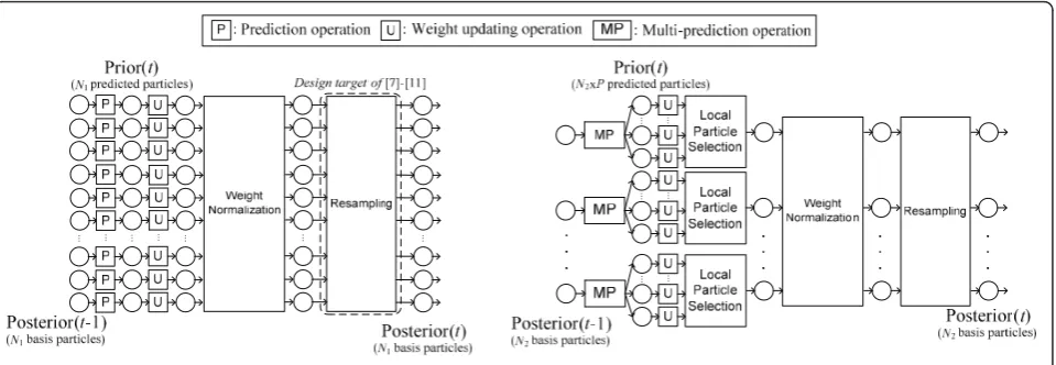
The conventional sequential importance resampling (SIR) PF is composed of four operations: (1)prediction, (2) weight updating, (3) weight normalization, and (4) resampling, as shown in Figure 1a. The prediction and weight updating steps form thesamplingprocedure, and the samplingprocedure is a data-independent operation and can be parallelized effectively. Since particle sam-pling is parallel in nature, many studies have explored and proposed parallel architectures for PF, especially by Bolićet al. [6,7]. However, the resampling procedure of the SIR-PF needs the weight information of whole parti-cle set and results in global data exchange. Hence, it suppresses the efficiency of the SIR-PF parallel imple-mentation. Recently, the idea of independent Metropo-lis-Hastings (IMH) algorithm [8] is utilized to facilitate the parallel design of the resampling procedure in PF [9,10]. In conclusion, to enhance the parallelized PF, the
* Correspondence: [email protected]
Department of Electrical Engineering, Graduate Institute of Electronics Engineering, National Taiwan University, Taipei, 106, Taiwan
studies in [7-11] focus on the modification of the resam-pling operation.
Based on the Amdahl’s law[12], the sequential por-tion of a task limits the speed-up in parallelized imple-mentation. The resampling procedure is a sequential task that significantly limits the acceleration of the par-allelized PF. In general, the complexity of the resampling procedure is proportional to the size of the posterior particle set. In tradition, the prior application domain knowledge can be utilized in the system model to reduce the uncertainty of the system state, such as [13,14]. However, this approach is application-dependent and hard to be utilized in other applications.
In this article, we propose a multi-prediction (MP) sampling approach to profit the parallelized PF. The proposed MP-sampling approach consists of MP opera-tion, weight updating, and local particle selecopera-tion, as shown in Figure 1b. In the proposed MP operation, multiple predicted particles are generated from a speci-fic basis particle, and the prediction number is defined asP. The SIR-PF withN1 basis particles can generate
N1 predicted particle. The proposed MP-PF with N2
particles can generateN2 ×Ppredicted particles. AsPis large, the required basis particle number of the pro-posed MP-PF can be significantly reduced for the same predicted particle number. Hence, the proposed MP-PF can suppress the complexity of the resampling proce-dure and benefit the parallelized PF. Besides, the pro-posed MP-PF has an overhead of additional prediction computations from the MP operation. Because the pre-diction procedure is data independent for each basis particle, the MP operation can be easily implemented in parallel. In summary, the proposed MP-PF reduces the sequential global data operation resulting from the resampling procedure by increasing the local computa-tion overhead. Hence, the proposed MP-PF improves
the execution time of the parallelized PF by reducing the complexity of the resampling procedure. It should be noted that our approach is not proposed to replace the algorithms in [7-11]. Proposed MP-PF can be com-bined with modified resampling algorithms in [7-11] to further improve the efficiency of the parallelized PF. To clarify the benefit of our approach, we compare pro-posed MP-PF with regular SIR-PF.
Recently, multi-core graphics processing units (GPUs) are popular in the signal processing domain [15-17] for its capability of massive parallel computation. The main feature of the multi-core GPUs is its high efficiency to process many parallel local computations. However, the latency of the memory access in GPU is much larger, because GPU does not have levels of cache for global data. If the executed task consists of many sequential operations or uncoalesed global data access [18], then the processing cores have to stall and result in low utili-zation. The proposed MP-PF trades additional local computations for reducing the amount of the global data access. To verify the benefit of the proposed MP-PFs, we implement the proposed MP-PF on NVIDIA multi-core GPUs. Our prototype results show that the proposed MP-PFs can be above 10× faster than the SIR-PF on multi-core GPU platform.
The rest of this article is organized as follows. The review of conventional SIR-PF is given in Section 2. Then the proposed MP-PF is presented in Section 3. The simulation results of the proposed MP-PFs are shown in Section 4. Implementation on the NVIDIA GPU and comparisons are presented in Section 5. Finally, Section 6 concludes the study of this article.
2. Review of SIR Pf
The basic procedures of the SIR-PF are briefly intro-duced in this section. System state transition model and
...
...
...
...
...
...
... ...
... ... ... ... ...
measurement model are two key models in the SIR-PF framework, as shown in Equations 1 and 2, respectively
xt =ft(xt−1,nt−1), (1)
yt=ht(xt,vt). (2)
where xtis the system state vector that we want to
track;ntthe random vector describing the system
uncer-tainty; ytthe observable measurement vector; andvtthe
measurement noise vector. The PF algorithm can work in the condition that ftand htare nonlinear or ntand
vtare non-Gaussian distribution. The PF algorithm needs
the following information about system x and observa-tiony:
•P(x0): The PDF of the initial system state.
•P(xt|xt-1): The transition PDF of system state.
• P(yt|xt): The observation likelihood function of
ytwith a given system state.
To track the current system state, the posterior PDFP (xt|y1:t) is required. Based on theBayes theorem,P(xt|y1: t) can be represented by likelihood function P(yt|xt)
transition prediction function P(xt|y1:t-1) and the
nor-malization termP(yt|y1:t-1):
P(xt|y1:t) =
P(yt|xt)P(xt|y1:t−1)
P(yt|y1:t−1) . (3)
From Equation 3, the prior prediction probabilityP(xt|
y1:t-1) can be represented as
P(xt|y1:t−1) =
P(xt|xt−1)P(xt−1|y1:t−1)dxt−1. (4)
For nonlinear/non-Gaussian scenario, Equations 3 and 4 cannot be obtained analytically. The SIR-PF approxi-mates the posterior P(xt|y1:t-1) with a particle set
{x(ti),w(ti)}N
i=1, andw (i)
t is associated weight for each parti-cle. The SIR-PF algorithm withNparticles is described as
Initialization
Generate Ninitial particlesx(1)0 , ...,x(0N)from pre-defined initial state distribution P(x0). All particles have equal initial weights,w(0i)= 1/N.
Iteration–Repeat fort= 1, 2, 3,...:
(a) Prediction: Draw the predicted particles x(ti) through the state transition model. For i = 1,...,N,n(ti) are independent with each other. These predicted parti-cles can be utilized to approximate the prior prediction distributionP(xt|y1:t-1).
(b)Weight updating: After receiving the measurement, each particle needs to update the weight according to the likelihood functionP(yt|x(ti)), as shown in Equation 5:
w(ti)=w
(i)
t−1·P(yt|x
(i)
t ). (5)
(c)Weight normalization: The normalization proce-dure makes the sum of particle weights equal to one. The particles with normalized updated weights can represent the posterior state distribution. The normali-zation procedure is represented as
w(ti)=w(ti)/
N
w(ti). (6)
(d)Resampling: After weight updating operation, some particle weights may be degenerated to a small value near zero. In general, systematic resampling (SR) is widely used for standard implementation of the resam-pling procedure. The SR procedure is to draw a new particle set with independent index j1,...,jNsuch that
P(jk=i)∝w(ti) and set xˆ( jk)
t =x(ti) Besides, all particle weights are set to 1/N.
The data flow of the SIR-PF with N1 particles is
shown in Figure 1a. The posterior particles at (t - 1) serve as the basis particles to generate the predicted prior particles att. There is a tradeoff between estima-tion accuracy and particle number. The SIR-PF with lar-ger Nwill increase the estimation accuracy. However, because the resampling operation is executed on the posterior particle set, the SIR-PF with largerNwill raise the complexity of the resampling operation.
3. Proposed MP PF algorithm
The data flow of the proposed MP-PF with N2 basis
particles andP predictions is shown in Figure 1b. Our proposed MP-PF is developed based on the SIR-PF. We replace the sampling procedure in the SIR-PF with our proposed MP-sampling approach. There are two modifi-cations in the proposed MP-sampling approach: (1)MP operation. (2)Local particle selection (LPS) operation.
3.1 Proposed MP operation
The proposed MP operation is inspired by the phenom-enon–unpredictable behavior of the target. Due to the uncertainty in the system transition model described by P(xt|xt-1), the state propagation has many, even infinite
operation, each basis particle makes multiple predictions according to the system model to track the uncertain system state. With the same number of basis particles, the MP-PF can produce a predicted prior particle set with larger size than the SIR-PF. Hence, the MP-PF can give more prediction state diversity to track the system state.
In the MP-PF,Plocal predicted particles are generated from one basis particle according to the system transi-tion model, as shown in Equatransi-tion 7
x(localj) ∼f(x(t−i)1, n(t−j)1), j= 1, 2, ..., P. (7)
x(t−i)1is a specific basis particle att- 1. The local pre-dicted particle set,{x(localj) }P
j=1,is a sample-based
represen-tation of transition PDF P(xt|x(t−i)1).In the predicted
prior distribution, each predicted particle has equal weight as well as equal importance, and none of the pre-dicted particles can be removed. After weight updating, the importance of each particle is not equal, and some local predicted particle with low importance can be removed. To maintain the same number of the basis particles for next iteration, the MP-sampling approach uses the LPS procedure to reserves only one representa-tive particle in each local particle set.
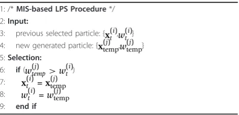
In each local particle set, only one particle has to be stored. For each basis particle, the local predicted parti-cles are generated sequentially, and we can avoid storing all local temporary particles. The pseudo code of the MP operation with M basis particles andP predictions is shown in Table 1. The previous selected particle and the new generate particle are inputted to the LPS proce-dure. The LPS procedure reserves a proper particle as the new selected particle based on their weights. It should be noted that the MP-PF is the same as the
SIR-PF as prediction numberP= 1. ForP> 1 with the same number of basis particles, the MP-PF can generate a lar-ger predicted prior particle set than the SIR-PF.
3.2 Proposed LPS mechanisms
From each basis particle, a group of predicted particles are generated. As mentioned above, the importance of each particle is not equal after weight updating. Hence, after weight updating, fewer particles need to be stored. In the proposed MP-sampling approach, the LPS proce-dure reserves one representative particle in each group. The representative particle is selected based on the weight distribution of the local predicted particle set. Two LPS approaches are described in the following. 3.2.1 Maximizing importance selection scheme
In each group of particles, the maximizing importance selection (MIS) scheme selects the particle with highest weight as the representative particle for this group, as described by Equation 8
indexselect= arg max
j=1∼P
(w(localj) ). (8)
Because the MIS scheme selects the particle with maximum weight in the local distribution, the MIS pro-cedure can be implemented sequentially. It should be noted that, for a widely used normal likelihood function, the MIS can select the representative particle based on the error distance rather than actual likelihood value. Therefore, for normal likelihood, the MIS needs only one likelihood calculation to update particle weight. Besides, the MIS scheme does not need a uniform ran-dom variable for selection procedure. The pseudo code of the MIS LPS procedure is given in Table 2.
3.2.2 Systematic resampling like selection scheme
The predicted particles from a specific basis particle can be regarded as a local distribution. In the systematic resampling like selection (SRS) scheme, the representa-tive particle is selected based on the SR algorithm. The SRS is a probabilistic selection scheme, and the prob-ability of jth local predicted particle being selected is defined by
Table 1 Pseudo code of the MP operation
1: /*Multi-Prediction Operation*/ 2:fori= 1 toNdo
3: x(1)temp∼f(x(i)
t−1,n (1)
t−1)//Generate 1
st
predicted particle
4: w(1)temp=w(i)
t−1·p(yt|x
(1)
temp)
5: x(ti)=x(1)temp
6: w(ti)=w(1)temp
7: forPredict countj= 2 toPdo 8: x(tempj) ∼f(x(i)
t−1,n (j)
t−1)
9: w(tempj) =wt(−i)1·p(yt|x(tempj) )
10: LPS(x(i)
t ,w
(i)
t ,x
(j)
temp,w
(j)
temp)
11: end for 12: end for
Table 2 Pseudo code of MIS-based LPS procedure
1: /*MIS-based LPS Procedure*/ 2:Input:
3: previous selected particle: {x(i)
t ,w
(i)
t }
4: new generated particle: {x(j)
temp,w
(j)
temp}
w(ti)=w
(j)
temp (9)
In general, the SR algorithm needs the cumulative sum information, and all predicted particles cannot be released until the SR procedure is accomplished. The conventional SR algorithm requires additional memory and processing latency. Fortunately, because the LPS procedure needs to select only one particle, the CDF scanning operation can be transformed to a sequential comparing operation. The detailed explanation is given in Appendix. The additional memory to temporally store the local particle set can be saved. Besides, the SRS procedure can start without waiting all local parti-cles are generated. This feature can increase the execu-tion efficiency of the SRS scheme. The pseudo code of the SRS LPS procedure is given in Table 3.
3.3 Prediction number and LPS scheme evaluation flow Before describing the evaluation flow, we analyze two LPS schemes first. There are two considerations for choosing LPS scheme:
3.3.1 Complexity
Both the SRS and MIS schemes are implemented by sequentialComparing-and-Replaceoperation. The differ-ence between two LPS schemes is the condition for replacing. The SRS scheme needs random variables to make a probabilistic selection. Besides, as mentioned above, the MIS scheme needs only one likelihood calcula-tion for normal likelihood. The complexity comparison between two schemes is given in Table 4. With the same setting of particle number and prediction number, the MIS scheme has lower complexity than the SRS scheme. 3.3.2 Robustness to measurement noise
In the SRS scheme, the representative particle is selected based on the PDF of the whole local predicted particle set. Hence, the predicted particles with similar weights have similar chance to be chosen as the representative particle in the SRS scheme. However, in the MIS scheme, the predicted particle with highest weight is
always selected as the representative particle. In sum-mary, the weights of the local particle set affect the result of the LPS procedure. In general, the measure-ment has a noise term. The weights of the particle set are updated based on the likelihoods to the measure-ment, so the weight is also affected by the measurement noise. As variance of the noise is high, the MIS scheme may suffer accuracy degradation, because the MIS scheme always selects the predicted particle with highest weight and believes the measurement too much.
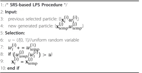
In summary, for target accuracy, we should evaluate both two schemes and select the scheme that has lower execution time. Prediction number Pand basis particle
numberNare main design parameters in the proposed
MP-PF. By increasing P, the MP-PF can reduce the
basis particle number as well as the global sequential operation. However, the total execution time may increase with too largeP. Therefore, for target accuracy, a proper setting of (N, P) and the LPS schemes should be evaluated for a specific parallel architecture.
Our suggested evaluation flow is shown in Figure 2. The prediction number set for evaluation and the target accu-racy should be predefined. For a specific prediction num-ber, the minimum particle number for the target accuracy can be obtained from simulation. With the prediction number and the particle number, the total execution time can be evaluated for a specific parallel architecture. We can obtain the setting of (N,P) with minimum execution time under the prediction number set. Eventually, we can choose a proper LPS scheme based on the minimum execution time of two LPS scheme.
4. Simulation results and discussion
The proposed MP-PF does not utilize the prior knowl-edge related to the application. In this section, we verify the proposed MP-PF by two widely used benchmark simulation models. In Section 4.1, we use a simple sys-tem transition model to evaluate the two LPS scheme at different measurement noise strength. In Section 4.2, we use the BOT model, which has high transition uncer-tainty to demonstrate the benefit of the proposed MP-PF.
4.1 Robustness to measurement noise
This model is highly nonlinear and is bimodal in nature. The system model and measurement model are described in Equations 8 and 9, respectively
xt=
xt−1
2 + 25·
xt−1 1 +x2
t−1
+ 8·cos(1.2t) +nt (10)
yt=
x2
t
20+vt (11)
Table 3 Pseudo code of the SRS-based LPS procedure
1: /*SRS-based LPS Procedure*/ 2:Input:
3: previous selected particle: {{x(i)
t ,w
(i)
t ,}
4: new generated particle: {x(tempj) ,w(tempj) ,} 5:Selection:
6: u~U[0, 1]//uniform random variable 7: w(ti)+ =w(1)temp
nt~ N(0,σn2), vt~ N(0,σv2). N(u,s2) is the normal
dis-tribution with meanu and variances2. The initial state distribution is x0 ~N(0,10). In our simulation, the var-iance of the system transition noise is set asσ2
n = 10.0.
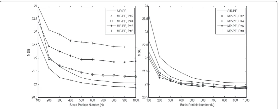
We take the weighted sum of posterior particles as the state estimation and calculate the mean-square-error (MSE) from the difference between the state estimation and the true state. The simulations are obtained from 104 randomly initialized experiments with 50 steps. To evaluate the robustness of the proposed LPS schemes, Figures 3, 4, and 5 give the MSE comparisons at differ-ent noise variance,σ2
v = 1, 1/4, and 1/16.
In this model, the term related to the hidden state is divide by 20, so the noise withσ2
v = 1is a large noise. In Figure 3, the MIS-based MP-PF suffers from huge accu-racy degradation due to high measurement noise, espe-cially for largeP. As the noise strength is large, the particle with highest weight is not perfectly correct. The represen-tative particle should be selected based on their probability distribution. However, the MIS scheme always selects the particle with highest weight in the local particle set, and this simple but hasty approach does not comply with the statistic of the local predicted particle set.
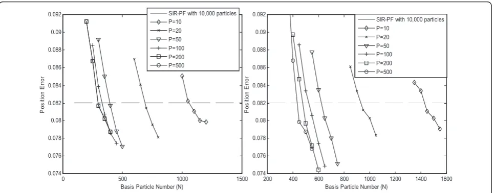
When the noise strength is lower, as shown in Figures 4b and 5b, the estimation accuracy of the MIS scheme can be improved. Nevertheless, the MIS scheme is still not robust to the measurement noise. Because the SRS scheme selects the representative particle in probabilistic
sense, the SRS scheme has better robustness to the mea-surement noise than the MIS scheme. The accuracy of the SRS scheme is always better than the SIR-PF, as shown in Figures 3, 4 and 5.
From Figures 3, 4 and 5, it is apparent that the SRS-based MP-PF has better estimation accuracy than the SIR-PF with the same basis particle number. In Table 5, we compare the SRS-based MP-PF and the SIR-PF with fixed number of predictions. The MSE performance of the SIR-PF converges around at particle numberN= 500. At this convergent point, we can give a fair comparison between the SRS-based MP-PF and the SIR-PF at the same total prior prediction number, 500. Table 5 gives the MSE com-parison results. AsN< 50, the proposed MP-PF has too few basis particles to sample the posterior PDF sufficiently. Although the MP approach can reduce the basis particle number, the basis particle number cannot be too small. With reasonable basis particle number, the proposed MP-PFs can give similar MSE results with much fewer basis particles. This result supports our clam that the proposed MP-PFs can reduce the memory requirement and the complexity of the resampling procedure.
4.2. The system model with high transition uncertainty In this section, we use the BOT model with high system transition uncertainty to further demonstrate the benefit of the proposed MP-PFs. In the BOT model, the state
vector include four state variables, i.
Table 4 Complexity comparison between the SRS and the MIS schemes
LPS scheme Distance calculation Likelihood computation Compare Div/Mul Generation of uniform R.V.
MIS P 1 (normal likelihood)P P- 1 0 0
SRS P P P- 1 P- 1 P
e.,xk=
PxkPykVxkVyk
T
. Following the Cartesian coordi-nate, the PxandPystand for the two-dimensional
posi-tion, whileVxand Vyare the two-dimensional velocity.
The observer is assumed to be at the origin, and the position as well as velocity are relative to the observer. The BOT system model is given in Equation 10
xk+1=Fxk+uk. (12)
where uk=
uxkuyk
T
∼N0,qI2
, and the matrices F andΓ are shown in Equation 11:
F=
⎛ ⎜ ⎜ ⎝
1 0 1 0 0 1 0 1 0 0 1 0 0 0 0 1
⎞ ⎟ ⎟
⎠, =
⎛ ⎜ ⎜ ⎝
0.5 0 0 0.5
1 0
0 1
⎞ ⎟ ⎟
⎠ (13)
The measurement is one-dimensional and consists of only bearing, i.e.,θk. We assume observer is fixed at the
origin, and the measurement model is illustrated in Equation 12
θk=h(xk) +vk= tan−1(
Pyk
Pxk
) +vk. (14)
where vk is additive Gaussian noise, and vk~N(0, r).
In our simulation,√q= 0.001and√r= 0.005, the same as the setting in [1]. We calculate the Position error from the difference between estimated position and the true position.
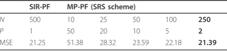
The position error results of the BOT model for two LPS schemes are shown in Figure 6. From Figures 3, 4 and 5, the proposed MP-PF can give a better perfor-mance than the SIR-PF, but the perforperfor-mance
100 200 300 400 500 600 700 800 900 1000
20.5 21 21.5 22 22.5 23 23.5 24
Basis Particle Number (N)
MS
E
SIR-PF MP-PF, P=2 MP-PF, P=4 MP-PF, P=6 MP-PF, P=8
100 200 300 400 500 600 700 800 900 1000
20.5 21 21.5 22 22.5 23 23.5 24
Basis Particle Number (N)
MS
E
SIR-PF MP-PF, P=2 MP-PF, P=4 MP-PF, P=6 MP-PF, P=8
Figure 3MSE results for different LPS schemes atσv2= 1..(a)MIS scheme;(b)SRS scheme.
100 200 300 400 500 600 700 800 900 1000
19 20 21 22 23 24 25
Basis Particle Number (N)
M
S
E
SIR-PF MP-PF, P=2 MP-PF, P=4 MP-PF, P=6 MP-PF, P=8
100 200 300 400 500 600 700 800 900 1000
19 20 21 22 23 24 25
Basis Particle Number (N)
MS
E
SIR-PF MP-PF, P=2 MP-PF, P=4 MP-PF, P=6 MP-PF, P=8
improvement is converged afterP= 6. Because the MP-sampling operation is utilized to track the uncertain sys-tem transition behavior, a huge number of predictions are not necessary in a simple model. However, in the BOT model, the SIR-PF needs thousands of particles to obtain good estimation accuracy. This phenomenon means that the BOT model has high system uncertainty, and the PF needs more particles to track the hidden state. In this condition, the MP operation can further give improvement by using larger P. In other words, in the system model with higher transition uncertainty, the number of basis particle can be reduced by using more predictions.
In Figure 6b, it is apparent that the MIS-based MP-PF has unstable behavior of the estimation accuracy. As the prediction number is large, the aforementioned draw-back of the MIS scheme is more apparent. Figure 7 gives the comparison results between two LPS schemes at different prediction number. For small prediction number, as shown in Figure 7a, two LPS schemes have similar estimation accuracy. With large prediction num-ber, as shown in Figure 7b, the SRS scheme can give better estimation accuracy than the MIS scheme due to its probabilistic selection mechanism.
As mentioned in Section 3, the MIS scheme selects the representative particle compulsorily. We can observe two drawbacks in the MIS scheme from the above
simulation: (a)low robustness to measurement noise; (b) the performance degradation in large prediction number. The drawbacks of the MIS scheme result from the sim-plification in the representative particle selection. The benefit of the MIS scheme is its simplicity. From the observation in simulation, the MIS scheme is feasible in low prediction number and low measurement noise. In contrast, the SRS scheme follows the posterior weight distribution to select the representative particle. Because the SRS select the local representative particle in prob-abilistic sense, the SRS scheme has higher stability and robustness than the MIS scheme.
5. Implementation of the MP-PFs on GPU 5.1. Parallelized MP-PF on NVIDIA multi-core GPU
The proposed MP-PF increases the prediction computa-tion to reduce the complexity of the resampling proce-dure. Because the MP-sampling operation can be executed independently among all basis particles, the prediction computation overhead can be compensated by parallel executions easily. In this subsection, we give the architecture of the MP-PF implemented on NVIDIA GPU. NVIDIA multi-core GPU can accelerate applica-tions with single-instruction-multiple-threads(SIMT) execution model and hierarchical memory.
As mentioned above, the MP-sampling procedure is independent among particles and can be parallelized by mapping each particle to parallel threads without efforts. Weight summation for normalization results in global memory accessing. For efficiency, shared memory can be utilized to buffer the intermediate data. In the resam-pling procedure, the global particle exchange needs uncoalesced global memory accessing [18], and this will
dominate the processing time to be near O(N) and
slower the resampling step significantly. The thread
100 200 300 400 500 600 700 800 900 1000
18 19 20 21 22 23 24 25
Basis Particle Number (N)
MS
E
SIR-PF MP-PF, P=2 MP-PF, P=4 MP-PF, P=6 MP-PF, P=8
100 200 300 400 500 600 700 800 900 1000
18 19 20 21 22 23 24 25
Basis Particle Number (N)
MS
E
SIR-PF MP-PF, P=2 MP-PF, P=4 MP-PF, P=6 MP-PF, P=8
Figure 5MSE results for different LPS schemes atσv2= 1/16.(a)MIS scheme;(b)SRS scheme.
Table 5 MSE comparison results at the same prediction number
SIR-PF MP-PF (SRS scheme)
N 500 10 25 50 100 250
P 1 50 20 10 5 2
block diagram of the SIR-PF is shown in Figure 8. Though with superior computing capability, the SIMT parallelism somehow suffers from inefficiency when pro-cessing uncoalesced global data exchange. The task with many global data transfer, like the resampling, will dom-inate the execution time on GPU.
5.2. Implementation result of the SIR-PF on GPU
To compare with the proposed MP-PFs, we first imple-ment the SIR-PF of the BOT model on a NIVIDIA GPU. The software interface for programming on NVI-DIA’s GPU is the compute unified device architecture (CUDA) [18,19]. The description of the GPU used in
this work is shown in Table 6. In Section 5.1, we described how to map the proposed MP-PF on NVIDIA multi-core GPU. For the SIR-PF, the only difference is the sampling procedure. As P= 1, the mapping in Sec-tion 3.4 is designed for the SIR-PF. Figure 9 shows the profiling results of the SIR-PF implemented on GPU, and the profiling data is the execution time of the PF with 25 iterations in the BOT model. The global opera-tions, the weight normalization and the resampling, indeed cost over 99% execution time while the sampling costs extremely little. Figure 9 validates that the resam-pling procedure dominates the execution time of the parallelized PF.
1000 2000 3000 4000 5000 6000 7000 8000 9000 10000 0.04
0.06 0.08 0.1 0.12 0.14 0.16 0.18 0.2 0.22
Basis Particle Number (N)
P
os
iti
on
E
rr
or
SIR-PF MP-PF, P=2 MP-PF, P=5 MP-PF, P=10 MP-PF, P=20 MP-PF, P=30
1000 2000 3000 4000 5000 6000 7000 8000 9000 10000 0.04
0.06 0.08 0.1 0.12 0.14 0.16 0.18 0.2 0.22
Basis Particle Number (N)
P
os
iti
on
E
rr
or
SIR-PF MP-PF, P=2 MP-PF, P=5 MP-PF, P=10 MP-PF, P=20 MP-PF, P=30
Figure 6Position error results for two LPS schemes.(a)MIS scheme;(b)SRS scheme.
1000 2000 3000 4000 5000 6000 7000 8000 9000 10000 0.045
0.05 0.055 0.06 0.065 0.07 0.075
Basis Particle Number (N)
P
os
iti
on
E
rr
or
MIS LPS SRS LPS
1000 2000 3000 4000 5000 6000 7000 8000 9000 10000 0.05
0.1 0.15 0.2
Basis Particle Number (N)
P
os
iti
on
E
rr
or
MIS LPS SRS LPS
5.3. Design example for loose target accuracy
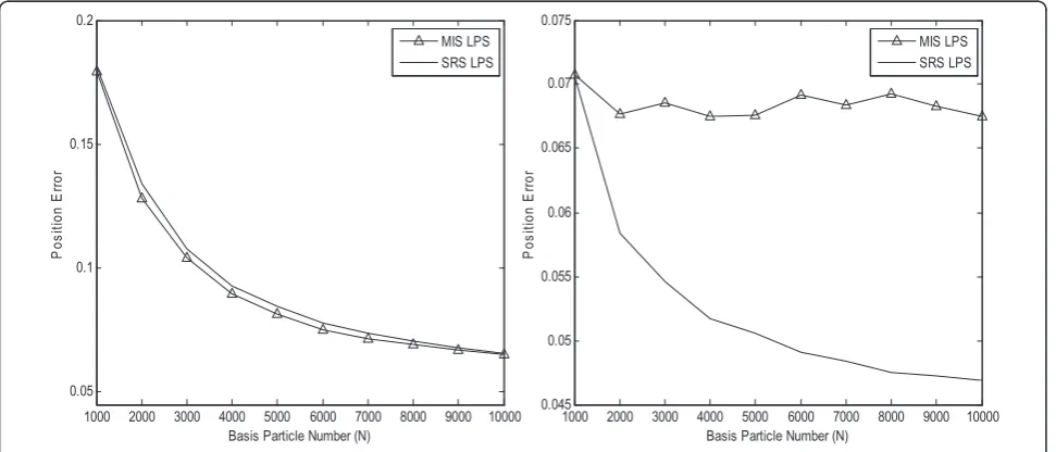
To compare with the SIR-PF, we set loose target accu-racy first, 0.08, which are simulated accuaccu-racy of the SIR-PF with 10,000 particles. The prediction number set for evaluation is {10, 20, 50, 100, 200, 500}. Figure 10 shows the estimation accuracy around the target accuracy. From Figure 11, the minimum particle number for each prediction number can be obtained. Table 7 illustrates the execution time and accuracy of the proposed MP-PF designs with different parameters. All parameter settings can meet the target accuracy 0.08.
The MP-PF can use hundreds of particles to meet the same estimation accuracy of the SIR-PF with 10,000 par-ticles. Besides, as the particle number is small, the parti-cle with higher weight may be more important to
represent the PDF, and the MIS scheme is a proper scheme for small particle number setting. Hence, the MIS MP-PF can use fewer particles than SRS scheme to achieve this accuracy threshold.
Figure 8Thread block diagram of the MP-PF on GPU.
Table 6 Hardware information for evaluation
GPU NVIDIA GeForce GTX 280
CUDA version 2.3
Number of SMs 30
Number of cores 240 Clock frequency 1.3 GHz
2000 3000 4000 5000 6000 7000 8000 9000 10000
0 100 200 300 400 500 600 700
Number of Particles, N
E
xec
ut
io
n t
im
e
(m
s)
Bearings-Only Tracking
(0.4%) Sampling & Weighting (14%) Weight normalization (85.6%) Resampling
The profiling results of the PFs listed in Table 7 are given in Figure 12. As shown in Figure 12, we can reduce the execution time of the resampling and the weight normalization procedure by using more predic-tions–larger P. However, when the particle number reduction slows down, largerPresults in execution time overhead of MP-sampling operation.
5.4. Design example for strict target accuracy
In the second design example, we set strict target accu-racy first, 0.06, which are simulated accuaccu-racy of the SIR-PF with 20,000 particles. The prediction number set for evaluation is {10, 20, 50, 100, 200, 500}, the same as in the above example. From the simulation result in Sec-tion 4.2, it should be noted that the MIS-based MP-PF is hard to achieve the threshold 0.06 with large P.
Therefore, for the accuracy threshold 0.06, the MIS MP-PF cannot use more predictions to reduce the execution time, and we skip the discussion of the MIS scheme for this target accuracy.
Figure 11 shows the estimation accuracy around the target accuracy. From Figure 11, the minimum particle number for each prediction number can be obtained. Table 8 illustrates the execution time and accuracy of the proposed MP-PF designs with different para-meters. All parameter settings can meet the target accuracy 0.06. Table 8 gives the proposed MP-PF designs that meet the second accuracy threshold. It should be noted that the MP-PF with the MIS scheme is hard to achieve the threshold 0.06 with largeP. The profiling results of the PFs listed in Table 8 are given in Figure 13.
0 500 1000 1500
0.074 0.076 0.078 0.08 0.082 0.084 0.086 0.088 0.09 0.092
Basis Particle Number (N)
P
os
iti
on E
rr
or
SIR-PF with 10,000 particles P=10
P=20 P=50 P=100 P=200 P=500
200 400 600 800 1000 1200 1400 1600
0.074 0.076 0.078 0.08 0.082 0.084 0.086 0.088 0.09 0.092
Basis Particle Number (N)
P
os
iti
on E
rr
or
SIR-PF with 10,000 particles P=10
P=20 P=50 P=100 P=200 P=500
Figure 10Comparison between the MP-PFs and the SIR-PF with 10,000 particles.(a)MIS scheme;(b)SRS scheme.
1 2 3 4 5 6 7
0 100 200 300 400 500 600
1:SIR-PF; 2~7:Proposed MP-PF
E
xec
ut
io
n t
im
e (
m
s)
N=10000
N=1450
P=10 N=950
P=20 N=650P=50 N=550P=100 N=500P=200 N=450P=500
Sampling Weight normalization Resampling
1 2 3 4 5 6 7
0 100 200 300 400 500 600
1:SIR-PF; 2~7:Proposed MP-PF
E
xec
ut
io
n t
im
e (
m
s)
N=10000
N=1100
P=10 N=650
P=20 N=400
P=50 N=350 P=100
N=300 P=200
N=300 P=500 Sampling Weight normalization Resampling
6. Conclusions
In this article, the MP framework with two LPS schemes is proposed to reduce the number of the basis particles. Among two proposed LPS schemes, the SRS scheme is robust to the measurement noise and does not suffer from accuracy saturation. The MIS scheme can work well for small prediction number Por particle number N. By reducing the basis particle number, the complex-ity of the resampling, the sequential part of the PF task, can be suppressed significantly. The MP framework increases the prediction computation, and this computa-tion can be easily implemented in parallel due to its data independent feature. In other words, the MP-PF
increases the overhead of the parallel task and reduces the complexity of the sequential task significantly. To demonstrate the benefit of the MP-PF for parallel archi-tecture, we implement the MP-PFs and the SIR-PF on multi-core GPU platform. For the classic BOT experi-ments, the maximum improvements of the proposed MP-PF are 25.1 and 15.3 times faster than the SIR-PF with 10,000 and 20,000 particles, respectively.
Appendix
Derivation of the proposed SRS scheme
Using the SR algorithm for selection, the probability of jth local predicted particle being selected as representa-tive particle is defined by
P(indexselect=j) = w(localj)
P i=1
w(locali)
, j= 1, 2, ..., P.
(15)
In general, the SR procedure needs to collect all pre-dicted particle information, and this results in additional latency and memory. Fortunately, the SRS procedure used in the proposed MP framework only selects one particle, and we modify the SR procedure into a sequential com-paring operation, as shown in Table 1, to save the memory and latency overhead. In the following, we demonstrate the proposed SRS scheme also follows the probability defined in Equation 14 to select the representative particle. For the MP operation withP prediction, the SRS can obtain a representative particle after (P- 1) probabilistic comparing test. The first predicted particle is set as initial representative particle. After passing (P- 1) com-paring test, the first predicted particle is accepted as final representative particle. The condition for first pre-dicted being the final representative particle is described as Equation 15
⎛ ⎜ ⎜ ⎜ ⎝
w(1)local
2
i=1
w(locali)
≥u1
⎞ ⎟ ⎟ ⎟ ⎠&
⎛ ⎜ ⎜ ⎜ ⎝
2
i=1
w(locali)
3
i=1
w(locali)
≥u2
⎞ ⎟ ⎟ ⎟ ⎠&...&
⎛ ⎜ ⎜ ⎜ ⎝
P−1
i=1
w(locali)
P
i=1
w(locali)
≥uP−1
⎞ ⎟ ⎟ ⎟ ⎠, (16)
Table 7 Execution time comparison between the MP-PF and the SIR-PF
N P Position error Execution time (speedup) SIR-PF
10000 1 8.2052 × 10⁻² 610.7 ms (1×) Proposed MP-PF (MIS)
1100 10 8.1061 × 10⁻² 67.7 ms (9.0×) 650 20 8.1426 × 10⁻² 41.1 ms (14.9×) 400 50 8.1702 × 10⁻² 27.0 ms (22.6×) 350 100 8.1376 × 10⁻² 24.8 ms (24.6×) 300 200 8.1692 × 10⁻² 24.3 ms (25.1×) 300 500 8.2049 × 10⁻² 36.8 ms (16.6×)
Proposed MP-PF (SRS)
1450 10 8.1067 × 10⁻² 89.9 ms (6.8×) 950 20 8.1225 × 10⁻² 58.9 ms (10.4×) 650 50 8.0923 × 10⁻² 44.0 ms (13.9×) 550 100 8.0021 × 10⁻² 41.8 ms (14.6×) 500 200 7.9687 × 10⁻² 44.7 ms (13.7×) 450 500 7.9891 × 10⁻² 59.8 ms (10.2×)
500 1000 1500 2000 2500 3000 3500
0.06 0.061 0.062 0.063 0.064 0.065 0.066
Basis Particle Number (N)
P
os
iti
on
E
rr
or
SIR-PF with 20,000 particles P=10
P=20 P=50 P=100 P=200 P=500
Figure 12Profiling results of the SIR-PF and the proposed MP-PFs with parameters shown in Table 5.(a)MIS scheme;(b)SRS scheme.
Table 8 Execution time comparison between the MP-PF and the SIR-PF
N P Position error Execution time (speedup) SIR-PF
20000 1 6.3124 × 10⁻² 1211.1 ms (1×) Proposed MP-PF (SRS)
where uiis an independent uniform random variable
forith probabilistic comparing test. Hence, the probabil-ity of first particle being accepted as representative par-ticle is shown as
P(indexselect= 1) =P ⎛ ⎜ ⎜ ⎜ ⎝ ⎛ ⎜ ⎜ ⎜ ⎝ w(1) local 2 i=1
w(locali) ≥u1
⎞ ⎟ ⎟ ⎟ ⎠& ⎛ ⎜ ⎜ ⎜ ⎝ 2 i=1
w(locali) 3
i=1
w(locali) ≥u2
⎞ ⎟ ⎟ ⎟ ⎠&...&
⎛ ⎜ ⎜ ⎜ ⎝
P−1
i=1
w(locali)
P
i=1
w(i) local
≥uP−1 ⎞ ⎟ ⎟ ⎟ ⎠ ⎞ ⎟ ⎟ ⎟ ⎠ =P ⎛ ⎜ ⎜ ⎜ ⎝ w(1) local 2 i=1
w(i) local
≥u1 ⎞ ⎟ ⎟ ⎟ ⎠·P
⎛ ⎜ ⎜ ⎜ ⎝ 2 i=1
w(i) local 3
i=1
w(i) local
≥u2 ⎞ ⎟ ⎟ ⎟ ⎠...·P
⎛ ⎜ ⎜ ⎜ ⎝
P−1
i=1
w(i) local
P
i=1
w(i) local
≥uP−1 ⎞ ⎟ ⎟ ⎟ ⎠ = w (1) local 2 i=1
w(locali) ·
2
i=1
w(i) local 3
i=1
w(locali) ·...·
P−1
i=1
w(i) local
P
i=1
w(locali)
= w (1) local P i=1
w(locali)
.
(17)
Thejth local predicted particle needs to pass (P-j+ 1) comparing test, and the accept probability is formed as
P(indexselect=j) =P ⎛ ⎜ ⎜ ⎜ ⎝
w(j) local
j
i=1
w(i) local
>uj−1 ⎞ ⎟ ⎟ ⎟ ⎠·P
⎛ ⎜ ⎜ ⎜ ⎝ j i=1
w(locali)
j+1
i=1
w(i) local
≥uj
⎞ ⎟ ⎟ ⎟ ⎠·...·P
⎛ ⎜ ⎜ ⎜ ⎝
P−1
i=1
w(locali)
P
i=1
w(locali) ≥uP−1
⎞ ⎟ ⎟ ⎟ ⎠ = w
(j) local
j
i=1
w(locali) ·
j
i=1
w(i) local
j+1
i=1
w(locali)
...·
P−1
i=1
w(i) local
P
i=1
w(locali)
= w
(j) local
P
i=1
w(locali)
.
(18)
From Equations 16 and 17, the SRS scheme follows the same probability described in Equation 14 to select the representative particle.
Acknowledgements
Financial supports from NSC (grant no. NSC 97-2220-E-002-012) are greatly appreciated.
Received: 1 February 2011 Accepted: 6 September 2011 Published: 6 September 2011
References
1. N Gordon, D Salmond, AF Smith, Novel approach to nonlinear/non-Gaussian Bayesian state estimation. IEE Proc F Radar Signal Process.140, 107–113 (1993). doi:10.1049/ip-f-2.1993.0015
2. A Doucet, N de Freitas, N Gordon (eds.),Sequential Monte Carlo Methods in Practice, Statistics for Engineering and Information Science(Springer, New York, 2001)
3. B Ristic, S Arulampalam,Beyond the Kalman Filter: Particle Filters for Tracking
(Artech House, Boston, 2004)
4. MS Arulampalam, S Maskell, N Gordon, T Clapp, A tutorial on particle filters for online nonlinear/non-Gaussian Bayesian tracking. IEEE Trans Signal Process.50(2), 174–188 (2002). doi:10.1109/78.978374
5. O Capp’e, SJ Godsill, E Moulines, An overview of existing methods and recent advances in sequential Monte Carlo. Proc IEEE.95(5), 899–924 (2007) 6. M Bolić,Architectures for Efficient Implementation of Particle Filters,(Ph.D.
dissertation, State University of New York, Stony Brook, August (2004) 7. M Bolić, PM Djurić, S Hong, Resampling algorithms and architectures for
distributed particle filters. IEEE Trans Signal Process.53(7), 2442–2450 (2005) 8. AC Sankaranarayanan, R Chellappa, A Srivastava, Algorithmic and
architectural design methodology for particle filters in hardware, inProc IEEE International Conference on Computer Design (ICCD), 275–280, (2005) 9. AC Sankaranarayanan, A Srivastava, R Chellappa, Algorithmic and
architectural optimizations for computationally efficient particle filtering. IEEE Trans Image Process.17(5), 737–748 (2008)
10. L Miao, J Zhang, C Chakrabarti, A Papandreou-Suppappola, A new parallel implementation for particle filters and its application to adaptive waveform design. inProc IEEE Workshop on Design and Impl Signal Proc Systems (SiPS), 19–24, (October 2010)
11. BB Manjunath, AS Williams, C Chakrabarti, A Papandreou-Suppappola, Efficient mapping of advanced signal processing algorithms on multi-processor architectures, inProc IEEE Workshop on Design and Impl Signal Proc Systems(SiPS-2008), 269–274, (October 2008)
12. MD Hill, MR Marty, Amdahl’s law in the multicore era. IEEE Trans Comput.
41(7), 33–38 (2008)
13. CH Chao, CY Chu, AY Wu, Location-constrained particle filter for RSSI-based indoor human positioning and tracking system, inProc IEEE Workshop on Design and Impl Signal Proc Systems(SiPS-2008), 73–76, (October 2008) 14. F Evennou, F Marx, E Novakov, Map-aided indoor mobile positioning
system using particle filter, inProc of IEEE Wireless Communications and Network Conf (WCNC), 13–17, (March 2005)
15. R Shams, P Sadeghi, RA Kennedy, RI Hartley, A survey of medical image registration on multicore and the GPU. IEEE Signal Process Mag.27(2), 50–60 (2010)
16. MD Bisceglie, MD Santo, C Galdi, R Lanari, N Ranaldo, Synthetic aperture radar processing with GPGPU. IEEE Signal Process Mag.27(2), 69–78 (2010) 17. NM Cheung, X Fan, OC Au, MC Kung, Video coding on multicore graphics
processors. IEEE Signal Process Mag.27(2), 79–89 (2010)
18. NVIDIA, NVIDIA CUDA TM programming guide, http://www.nvidia.com/ object/cudahomenew.html
19. E Lindholm, J Nickolls, S Oberman, J Montrym, NVIDIA Tesla: a unified graphics and computing architecture. IEEE Micro.28(2), 39–55 (2008)
doi:10.1186/1687-6180-2011-53
Cite this article as:Chuet al.:Multi-prediction particle filter for efficient parallelized implementation.EURASIP Journal on Advances in Signal Processing20112011:53.
1 2 3 4 5 6 7
0 200 400 600 800 1000 1200
1:SIR-PF; 2~7:Proposed MP-PF
E xec ut ion t im e (m s) N=20000 N=3050 P=10 N=2000
P=20 N=1400P=50 N=1150
P=100 N=1050P=200 N=950P=500
Sampling Weight normalization Resampling