EFFECTS OF DENSITY DIFFEHENCES ON 'LATERAL MIXING IN OPEN-CHANNEL FLOWS
Thesis by
Edmund Andrew Prych
In Partial Fulfillment of the Requiren1ents ·For the Degree of
Doctor of
Philosophy-California Institute of Technology ·Pasadena, California
1970
-ii
-/\t :1' NOWLED< i.EM ENTS
This st:udy, one of a group of invcsti gatious al. the Californi ;t Institute uf Technology titled "Dispersion in Hydrologic and Coastal Environments", was funded by the Federal w·ater Pollution Control Administration through Grants No. 16000 DGY and No. 16070 DGY. During the study the writer also received financial assistance in the form of stipends and tuition payments while a U.S. Public Health .Scrv.i ce 'I' r ai nee (l 96 7 -70) and while a National Science Foundation Trainee (19(16-67). The writer thanks each of these agencies for their s11 pport.
To Dr. Norrnan H. Brooks, adviser and fruitful source of 11the right questions 11
, the writer expresses his sincere gratitude. The writer also thanks Dr. Vito A. Vanoni for comments made during the study, and Dr. E. John List for his comments during the writing of
this thesis.
For their assistance in constructing and modifying laboratory equipn1ent, the writer offers a hearty thanks to Mr. Elton F. Daly, s11pc'rviso1· of the shop and laboratory; to Mr. Robert L. Greenway, his ta]enlt·d assistant; and to Mr. Carl A. Green, Jr. , who also pre
-111-performed a variety of tasks during this investigation; they are: l'vfcssrs. Raul Basu, George Chan, Yoshiaki Daimon, Edward F.
-iv-ABSTRACT
This study investigates lateral rnixing of tracer fluids in
turbulent open-channel flows when the tracer and an1bicnt fluids have different densities. Longitudinal dispersion in flowo with longitudinal density gradients is investigated also.
Lateral mixing was studied in a laboratory flume by introducing fluid tracers at the ambient flow velocity continuously and uniformly across a fraction of the flume width and over the entire depth of the ambient flow. Fluid samples were taken to obtain concentration distributions in cross-sections at various distances, x, downstream from the tracer source. The data were used to calculate variances of the lateral distributions of the depth-averaged concentration. When there was a difference in density between the tracer and the ambient fluids, lateral mixing close to the source was enhanced by density-induced secondary flows; however, far downstream where the density
gradients were small, lateral mixing rates were independent of the initial density difference. A dimensional analysis of the problem and the data show that the normalized variance is a function of only three dimensionless numbers, which represent: (1) the x-coordinate,
-v-to this velocity distribution was also obtained. Using this dispersion coefficient in an analysis for predicting lateral mixing rates in the experiments of this investigation gave only qualitative agreernent with the data. However, predicted longitudinal salinity distributions in an
Chapter
1.
2.
3.
V l
-TABLE OF CONTENTS
INTRODUCTION 1. I Purpose
1. 2 Method of Investigation
BACKGROUND AND REVIEW OF PREVIOUS WORK 2. 1 The Conservation Equation
2. 2 Mass Transport in Open-Channel Flows of Homogeneous Density
2. 2. 1 Longitudinal Dispersion 2. 2. 2 Longitudinal Diffusion 2. 2. 3 Lateral Diffusion
1
I 2
5
5
6
6 8 10 2. 2. 3. 1 Diffusion at the Free Surface 10 2. 2. 3. 2 Depth-Averaged Diffusion
Coefficient 10
2. 2. 4 Vertical Diffusion 15
2. 3 Effects of Density Differences on Mass Transfer 16 2. 3. 1 Vertical Density Gradients 16 2. 3. 2 Horizontal Density Gradients 17
EXPERIMENTAL APPARATUS AND TECHNIQUES 20
3. 1 Description of Experiments 20
3. 2 Flume 21
Chapter
4.
3. 3
3. 4
-vii-TABLE OF CONTENTS (Cont'd)
3. 2. 2 Water Circulation 3. 2. 3 Rough Bottom
Watc1· D<·pth and Velocity McaH11ring Eq11ip:r11enf: Tracer Fluid System
3. 4. 1 Fluid Handling System 3.4.2 Sources
21
24
?,(, 26
26
28
3.4.2. 1 Narrow Sources 28
3. 4. 2. 2 The Intermediate Width Sources 31
3. 4. 2. 3 Wide Source 33
3. 5 Fluid Sampling Apparatus 3. 6 Sample Analysis
3. 7 3. 8
3.9
3. 6. 1 Description of the Technique 3. 6. 2 Accuracy of the Technique Measurements of Fluid Density Experimental Procedures
3. 8. 1 3. 8. 2
3. 8. 3
Preparation
Positioning the Sampling Tubes Taking the Samples
Experiments With Floating Particles 3. 9. 1 Apparatus
3.9.2 Procedures
EXPERIMENT AL DAT A 4. 1 Hydraulic Data
35 38 38 42 43 45
45
46
47 49 49 51
-viii-TABLE OF CONTENTS (Cont'd)
Chapter
4. 1. 1 Flow Condition Code and Flume Bottom 5 4
4. 1. 2 Water Depth S4
4. 1. 3 Slope 56
4. 1. 4 Shear Velocity 58
4. 1. 5 Metered Discharge and Discharge
Velocity 58
4. 1. 6 Velocity in Central 60 cm of Flume 58
4. 1. 7 von Karman1s k 59
4. 1. 8 Friction Factors 62.
4. 1. 9 Reynolds Number and Froude Number 62 4. 2 Experiments With Fluid Tracers 63
4. 2. 1 Introduction 63
4. 2. 2 Concentration Distributions in
Cross-Sections 65
4. 2. 3 Depth-Averaged Concentration
Distributions 79
4. 2. 3. 1 Calculating the
Depth-Averaged Concentrations 79 4. 2. 3. 2 The Lateral Distributions of
C
804. 2. 4 Variances of the Lateral Concentration
Distributions 95
4. 2. 4. 1 Calculations of the Variances 95
4. 2. 4. 2 Presentation of the Variances 103
Chapter
5.
6.
-ix-TABLE OF CONTENTS (Cont'd)
4. 3 Experiments With Floating Particles 4. 3. 1 Calculating the Variance
4. 3. 2 Presentation of Data
DAT A ANALYSIS
Page
135
135
140
145
5. 1 Experiments Without Density Differences 145 5. 1. 1 Experiments With Tracer Fluids 145
5. 1. 2 Experiments With Floating Particles 147 5. 2 Experiments With Density Differences 149
5. 2. 1 Introduction 149
5. 2. 2 Selection of Dimensionless Numbers 149 5. 2. 3 The Dimensionless Variance 152
5.2.3. 1 The Excess Variance 5. 2. 3. 2 The Fraction r
153
160
5. 2. 3. 3 Maximizing Lateral Mixing 163 5. 2. 4 The Average Coefficient of Variation 166
5. 2. 5 Predicting Concentration Distributions 168
ANALYTIC STUDY 6. 1 Introduction 6. 2 Basic Equations
6. 3, Simplification of the Basic Equations 6. 3. 1 Lateral Mixing
6. 3. 2 Longitudinal Mixing
170
170
170
173
173
-x-TABLE OF CONTENTS (Cont'd) Chapter
6. 4 Solution for the Velocity w and the Dispersion
Coefficient Dz 18 1
6. 5 Application of Theory to Experiments of This
Study 186
6. 5. 1 Sources of Finite Width 186 6. 5. 2 Two Wide Parallel Streams 191 6. 6 Application of Theory to MIT Experiments 193 6. 6. 1 Description of Experiments 193
6. 6. 2 Theoretical Analysis of Experiment 196 6. 6. 3 Comparison of Theory With Experiment 198
7. SUMMARY OF RESULTS 204
7. 1 Experiments 204
7. 1. 1 Experiments Without Density 204 Differences
7. 1. 2 Experiments With Density Differences 205
7. 2 Theory 207
LIST OF SYMBOLS 209
LIST OF REFEHENCES 214
Nun1ber
") 1
3. 1
3. 2
3.4
3. 5 3. 6 3. 7
3.
8
3.
9
3. l 03. 11
3. 12
4. 1
4.2
-·
Xl-LIST OF FIGUHES
Description
Longitudinal pressure gradients and velocity distributions in an estuary
The 40-n1cter flun1e
Photograph of expanded metal lath used for
roughness on the bottom of the flume
Dirnensioned sketch of metal lath used for roughness on the bottom of the flume
Schematic drawing of the tracer-fluid handling system
The 1-cm-wide source
The 20-cm-wide source
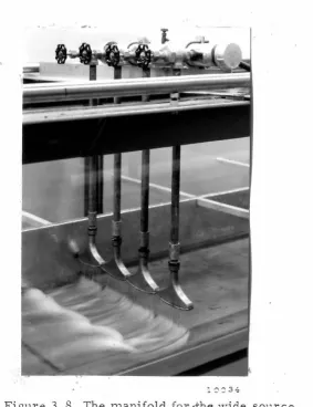
Photograph looking down the flume The m.anifold for the wide source
A fluid sampling rake
The pressure box and sampling rakes on the instrument carriage
Sample of polyethlene particles used in study of
lateral diffusion at the free surface
Compartmented-sieve particle collector; the compartments are 1 cm wide
Profiles of the energy grade line, water surface,
and flume bottom for flow S2
Cross -sections of the flume showing isovels 25 meters downstream from the flume inlet
Pa~c
·---""'-'·
-xii-LIST OF FIGUHES (Cont'd)
Nun1ber Description Page
4. 3 Velocity profiles observed 25 meters downstream
from the flume inlet 6 l
4. 4 Lines of equal relative concentration in
cross-sections downstream from a 1-cm-wide source
which discharged a fluid with a density the same as the
ambient fluid and with a relative concentration of 1. 0. 67
4. 5 Lines of equal relative concentration in
cross-sections downstream from a I-cm-wide source
which discharged a fluid with a density 0. 0160 gm/cm3
greater than the ambient fluid and with a relative
concentration of l. 0 68
4. 6 Lines of equal relative concentration in
cross-sections downstream from a I-cm-wide source
4. 7
4. 8
4
.
9
4. 10
4. 11
4. 12
which discharged a fluid with a density O. 0158 gm/cm3
less than the ambient fluid and with a relative
concentration of 1. 0
Cross-section of flume showing density-induced secondary circulation patterns downstream from a source of narrow or intermediate width
Cross -sections with lines of equal relative
concentration downstrea:rn from the confluence
of two wide parallel strea:rns of the same density
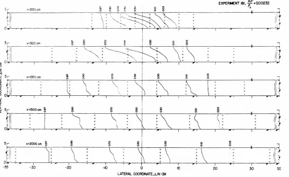
Cross-sections with lines of equal relative
concentration downstream from the confluence
of two wide parallel streams of different density
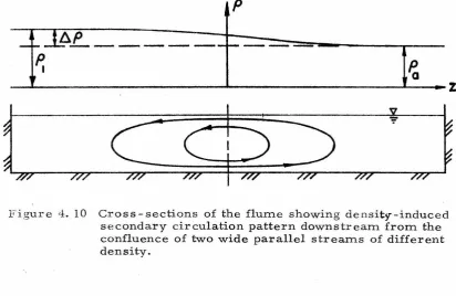
Cross-sections of the flume showing dens
ity-induced secondary circulation pattern downstream
from the confluence of two wide parallel streams
of different density
Definition sketch for terms in Eq. 4. lb
Depth-averaged concentration distributions
down-stream from a I-cm-wide source which discharged
a fluid with a density the same as the ambient fluid
and with a relative concentration of 1. O; Exp. 125
69
71
76
77
78
80
Number 4. 13
4. I4
4. I5
4. I6
4. 17
4. I8
4. 19
4.20
4. 2 I
4.22
-xiii--LIST OF FIGURES {Cont'd)
.Description Page
Depth-averaged concentration distributions down-stream from a I-cm-wide source which discharged a fluid with a density the same as the ambient fluid
and with a relative concentration of 1. O; Exp. l I6 83 Depth-averaged concentration distributions down
-stream from a I-cm-wide source which discharged a fluid with a density 0. 0160 gm/ cm3 more dense than the ambient fluid and with a relative concen
-tration of 1. O; Exp. I I3 84
Depth-averaged concentration distributions dow n-stream from a I-cm-wide source which dischar ged a fluid with a density 0. 0158 gm/cm3 less than the ambient fluid and with a relative concentration of
1. 0; Exp. 128 85
Depth-averaged concentration distributions d own-stream from a 20-cm-wide source which discharged a fluid with a density the same as the ambient fluid
and with a relative concentration of 0. 0370; Exp. 150 88 Depth-averaged concentration distributions
down-stream from a 20-cm-wide source which discharged a fluid with a density O. 00186 gm/ cm3 more dense than the ambient fluid and with a relative concen
-tration of O. 0385; Exp. 152 89
Depth-averaged concentration distributions down -stream from the confluence of two wide parallel
streams of the same density; Exp. 177 91 Depth-averaged concentration distributions dow
n-stream from the confluence of two wide parallel
streams of different density; Exp. 181 92 Depth-averaged concentration distributions, on
arithmetic probability paper, downstream from the
confluence of two wide parallel streams; Flow Sl 94 Cumulative distributions of depth-averaged
concentrations from Exp. 125, f).p/ p = 0 102
a
a) Variance- and b) Coefficient of vari ation-distance curves from experiments with flow SI
Number 4. 23 4.24 4. 25 4.26 4.27
4. 28
4.29 4.30 4. 31 4.32 4.33 4.34
-xiv-LIST OF FIGURES (Cont'd) Description
a) Variance- and b) Coefficient of variation-distance curves from experiments with flow S 1 and the 12. 5-cm-wide source
a) Variance- and b) Coefficient of variation-distance curves from experiments with flow S 1
and the 20-cm-wide source
a) Variance- and b) Coefficient of variation-distance curves from experiments with flow S 1 and the 10-cm-wide source
a) Variance- and b) Coefficient of variation-distance curves from experiments with flow S 1 and the wide source
a) Variance- and b) Coefficient of variation-distance curves from experiments with flow S2 and the 1-cm-wide source
a) Variance- and b) Coefficient of variation-distance curves from experiments with flow S2 and the 20-cm-wide source
a) Variance- and b) Coefficient of variation-distance curves from experiments with flow S3 and the 1-cm-wide source
a) Variance- and b) Coefficient of variation-distance curves from experiments with flow R 1 and the 1-cm-wide source
a) Variance- and b) Coefficient of variation-distance curves from experiments with flow R 1 and the wide source
a) Variance- and b) Coefficient of variation-distance curves from experiments with flow R2 and the 1-cm-wide source
a) Variance- and b) Coefficient of variation-distance curves from experiments with flow R2 and the 20-cm-wide source
Photographs of experiments with flow S 1 and the I-cm-wide source
-xv-LIST OF FIGURES (Cont'd)
Number Description Page
4. 35 Photographs of experiments with flow R l and the
1-cm-wide source 121
4. 36 Photographs of experiments with flow S l and the
20-cm-wide source 123
·l. 3 7 Photographs of experiments with flow S2 and the
l-cn1-wide source 124
4. 38 Photographs of experiments with flow R 1 and the
wide source 125
4. 39 Photographs of experiments with flow S 1 and the
wide source 126
4. 40 Vertical concentration distributions downstream from a 1-cm-wide source which discharged a fluid with a density the same as the ambient fluid and with a relative concentration of 1. O; flow S2;
Exp. 116 130
4. 41 Vertical concentration distributions downstream from a I-cm-wide source which discharged a
fluid with a density 0.0160 gm/cm3 greater than the ambient fluid and with a relative concentration
of 1. O; flow S2; Exp. 113 131
4. 42 Vertical concentration distributions downstream from a I-cm-wide source which discharged a fluid with a density 0. 0158 gm/cm3 less than the
ambient fluid and with a relative concentration
of 1. O; flow S2; Exp. 128 132
4. 43 Vertical concentration distributions downstream from the confluence of two wide parallel streams
of the same density; flow S 1; Exp. 177 133 4. 44 Vertical concentration distributions downstream
from the confluence of two wide parallel streams
of different density; flow SI; Exp. 181 134 4. 45 Cumulative distributions of particles; a) Exp. 102,
b)Exp.101 136
Nun1ber
4.48
-:!. 49
4.50
5. 1
5. 2
5. 3
5.4
-xvi-LIST OF FIGURES (Cont'd) De::>cription
Variance -dis ta nee curves for experirn<'nts with
floating particles; flow SI
Variance-distance curves for experinit~nts w.ith
floating particles; (a) flow S2, and (b) flow S3
Variance-distance curves for experiments with
floating particles; (a) flow R 1, and (b) flow R2 Definition sketch for r and b.V
The dimensionless excess variance, D,V, as a function of the dimensionless source strength, Mb, and the dimensionless source width, B
The ditnensionless excess variance, D.V, as a function of the dimensionless source strength,
Md, and the dimensionless source width, B
The intercept, Mt, as a function of the diinensionless source width, B
5. S The fraction of the excess variance, r, as a
function of the dimensionless distance down
-stream, X
5.
6
a) Variance-, and b) Maximun1concentration-distance curves from some experiments with simi).ar flow conditions and values of Mb but different source widths
5. 7 Laterally averaged coefficient of variation, C , as a function of the dimensionless distance v
6.
16. 2
6.3
6.4
downstream, X
Theoretical velocity profiles, w(11) with
w
:.:
0, for three different sets of boundary conditionsComparison of /:,.V given by Eq. 6. 42 and by experiment
Schematic diagram of the flume used in the MIT experiments (Ref. 2)
Solutions to Eq. 6. 61, -C - dC
+
J fdC) 3-
·
as
\d
s
-xvii-LIST OF FIGURES (Cont'd)
Number Description
6. 5 Depth-averaged relative concentration C as a function of
s
,
the dimensionless longitudinal coordinate; for MIT Runs 21 to 246. 6 The dimensionless distance s~~ as a function of the parameter J
200
-xviii-LIST OF TABLES
Nun1ber Description
2.. I Sum.mary of published data on longitudinal diffusion of floating particles in open-channels 2.2
2.3
3. 1
3.2
3. 3
4. 1 4.2
4.3
4.4
5. 1
6. 1
Al
Summary of published data on lateral diffusion of floating particles in open-channels
Summary of published data on lateral diffusion of solutes in open-channels
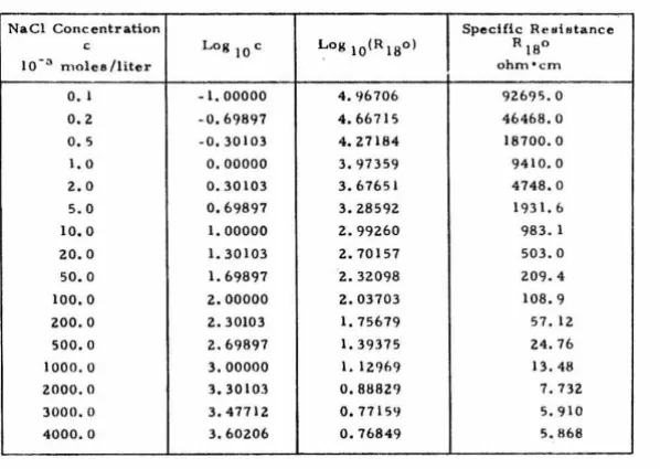
Specific resistance at 18°C as a function of NaCl concentration
Data from tests to check accuracy of technique for determining relative concentrations
Probability that the error in
cr
2is exceeded as a function of the number of pafticles collected Sumr:nary of hydraulic data
Li st of experiments with tracer fluids Sample table from Ref 1
Variances of lateral distributions of depth-averaged concentrations in Exp. 125
Lateral turbulent diffusion coefficients from this study
Coefficients in Eq. 6. 30 and 6. 31 for w(T]) and D z Summary of data from experiments with the 1-cm-,
12. 5-cm -, and 20. 0-crn-wide sources
AZ Summ.ary of data from experiments with the wide source
l
-CHAPTER 1
INTRODUCTION
1. 1 PURPOSE
Many waste effluents which are discharged into streams have densities slightly different from those of the receiving waters. This study investigates the effects of density differences on the horizontal, cross stream mixing of such effluents. Longitudinal mixing under certain restrictive conditions is also examined.
Two typical cases in which the effluents and the receiving waters have different densities are: heated cooling water discharges from industries or steam power plants, and domestic or industrial waste
discharges into brackish estuary waters. In the case of the cooling water discharges, a temperature difference of 10°C causes a density difference of approximately 0. 25 percent. In the second case, a waste discharging into an estuary, the density differences due to differences is concentrations of dissolved salts can be as high as 2. 5 percent. In both these cases the densities of the effluents are less than that of the receiving waters.
-2-of dis solved matter that are discharged into fresh water streams,
and alsn waste discharges with suspensions of fine particulate matter
t Ii at. i:.; 1nore dense than water. Density differences dne to
con-centration::; of dissolved or suspcn<led 1nattl~r can range up to a few
percent, although'. a fraction of a percent may be h1ore typical.
Alt.hough the magnitude of the density differences gi vcn above
n.1ay secni sn1all, differcncc~s of these magnitudes and snialler often
have large effects on the dynamics of oceans, lakes and the
atmosphere. This study investigates their importance in streams.
1. 2 METHOD OF INVESTIGATION
In this study the effects of density differences on cross stream
n1ixing were studied experimentally in a laboratory flume. In the
c;-.;pednients, which are described in Chapter 3, tracer fluids with
densities equal to and slightly different from the density of the
;:rn1bicnt water in the flunH'! were introduced over some part of the
width and uniformly over the whole depth. If the tracer and
arnbient fluids have the same density, ;crosswise mixing is primarily
by turbulent diffusion. However, if the densities of the tracer and
ambient fluids are different, crosswise mixing is enhanced by a
density-induced secondary flow. The forces driving the secondary
flow arc due to an inbalance of hydrostatic pressure caused by lateral
cknsity gradients. The phenomenon of density-induced circulation is
d Lscussed in more detail in the literature review of Chapter 2 and in
.
,
-· '
-So111t· of t.111~ clcd .. l, sliuwing l:ht: charact:ori.:~t:ic r~.·-d.111·c11 of the c,>11~cntt·d.tion di::;triliution:-; obsc1·ved in the t•xperin1e11ts, arc given in Chapter 4. The concentrations n1easured at all points in all
experin1ents are made available in Ref. 1, but they are not included in this text because the data are too numerous.
A dimensional analysis of the problem of lateral mixing in
an open channel is given in Chapter 5. The results of the analysis and the experimental data yield empirical curves for parameters which
characterize the tracer-plume width and the variation of concentration
wi l:h depth as fnnctions of distance downstrcan1 frorn tl1e source, the
ini lial density difference, the source width, and the hydraulic
para1neters of the stream. Concentration distributions can be
estimated by using these curves.
A simplified theory for the effect of horizontal density gradients on horizontal mixing is given in Chapter.
6.
The velocity distributionc:.:i..used by a horizontal density gradient was derived, and an
e:~pression for the dispersion coefficient due to the density-induced velocity was calculated. An analysis using this dispersion coefficient
p1·edicb: that the characteristic width of a tracer plurn1· in a.n open
were obtained from the diinensional analysis and data. However,
because some of the simplifying assumptions rnade in the derivation of
-4-The approximations in the derivation of the density-induced velocities are more nearly correct for some experiments in an idealized
-5
-·CHAPTER 2
BACKGROUND AND REVIEW OF PREVIOUS WORK
)
,
_
.
Tl! E CONSEHV ATION EQUATION.In most n1athematical analysis of turbulent flows, the transport
of solutes or other tracers is often described by an appropriate
time-averaged conservation equation for the tracer. The equation usually
used for aqueous solutions, which are nearly incompressible but not
necessarily of uniform density, is
(2. 1)
(see e. g. Harleman (3)). In this expression, tis time; c is a time
-avcra.µyd concentration: u, v, and w arc tin1c-averagcd velocitie8 in
the rc•cl:ilinear coordinate directiorrn, x, y, and :1.; a11d e , r-: , and ,.;
x y z
a:re turbulent diffusion coefficients for mass. (The velocities and
concentrations in Eq. 2. 1 are averages over a time that is long
compared to the time scale for turbulence, but short compared to
the time scale for the gross phenomena being investigated. )
If the density of the fluid is a function of c, then u, v, w,
E: and r:: may be functions of c also. Under these conditions,
'y' z
€ ,
x
Eq. 2. 1 is nonlinear in c and must be solved simultaneously with
-6-does not affect the dynamics of the flow, Eq. 2. I is linear in c and the equations of n1otion for the fluid n1ay be solved separately. However, even under these simplified conditions, analytic solutions for Eq. 2. 1 have been obtained only for very simple flow fields.
Below, a review is given of existing information on mass transport in turbulent open-channel flows of homogeneous density. It is followed by a discussion of the effects of density differences on mass transport.
2. 2 MASS TRANSPORT IN OPEN-CHANNEL FLOWS OF HOMOGENEOUSDENfilTY
2. 2. 1 Longitudinal Dispersion.- The coordinate system for an open channel flow is chosen with the origin on the channel bottom, the x-axis in the direction of flow, the y-axis normal to the bottom
and positive upwards, and the z-axis horizontal and in the lateral direction. For a uniform steady flow of a fluid of uniform density in a wide channel of uniform depth, v
=
w= o,
and ae:I
ax
=ae
I az
=o.
x z
For these conditions, Eq. 2. 1 becomes
(2. 2)
One now substitutes into Eq. 2. 2 the expressions: u =
u
+
u'c
=
c
+
c'
-7-where the overbarred quantities are depth-averaged variables and the primed quantities denote deviations from the averages. Averaging the resulting expression over the depth, and recognizing that
au I
I
ox
::::
O, yields(2. 3)
The second term on the left-hand side of Eq. 2. 3 represents
differential convection by the mean velocity,
u,
and the third term represents differential convection due to the correlation between u'and c'. Elder (4) showed that for two-dimensional flows in which
fk/oz
=
O, one can write for large timeu'c'
=
-D Ilex
ax '
(2. 4)where D is called the longitudinal dispersion coefficient.
x He showed
that D is only a function of u' and € and is given by
x y
1 T\ T\1
Dx
=
-d2J
u' (T))J
€ tri•)J
u' (T\11) dT) dri'd
n"
,
0 0 y 0
(2. 5)
where T), ri', and T)11 are y Id. Using the Prandtl-von Karman
logarithmic velocity distribution to obtain u' and the Reynolds analogy to obtain € (see Subsection 2. 2. 3 ), Elder integrated Eq. 2. 5 to
y give
where k is von Karman's constant; u* is the shear velocity, and d
(2. 6)
-8-2. -8-2. 2 Longitudinal Diffusion. Because transport by longitudinal
dispersion, as described above, and transport in the longitudinal
direction by turbulent diffusion are additive, and because D
>
>
E:x x'
little experimental data on e exist.
x
Data on longitudinal diffusion at the free surface are available
from experiments by Sayre and Chang (5) and by Engelund (6 ). In
these studies, small floating particles were released at a point on
the free surface, and either the distribution in time for particles to
travel a fixed distance or the longitudinal distribution of particles
after a fixed time from release were observed. Longitudinal
turbulent diffusion coefficients at the free surface,
e
,
were XScalculated using
E:
XS (2. 7 a)
or
(2. 7b)
where cr~ and CJ~ are the variances of the distributions of the particles
m space and time, and u is the mean longitudinal particle velocity.
s
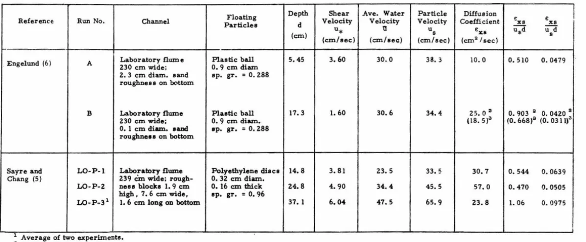
Sayre and Chang normalized E:xs by dividing by u,;,d, but
Engelund chose to divide his coefficients by u d. Both normalizations s
were made on both sets of data and the results are given in Table 2. I.
Neither normalization of the published data give·s more consistent results
than the other; however, using the re-evaluated coefficient for Engelund1s
Run B, which is obtained by recomputing E: from his published basic xz
data, the normalization by u,~d gives slightly more consistent results.
Normalization by U:*d is also more appropriate because u,." characterizes
Table 2. 1 Summary of published data on longitudinal diffusion of floating particles in open channels.
Reference Run No. Channel
Engelund (6) A Laboratory flume
230 cm wide; 2. 3 cm diam. eand
roughneu on bottom
B Laboratory flume
230 cm wide; O. l cm diam. •and roughneu on bottom
Sayre and LO-P-1 Laboratory flume
Chang (5) 239 Cm wide;
rough-LO-P-2 neu blodte 1. 9 cm
LO-P-31
high. 7. 6 cm wide, l. 6 cm long on bottom
1 Average-;;! two eJl:l>erimente. a Published data.
3 Re-evaluated data.
Floating Depth Velocity Shear Particles d
u* (cm)
(cm/sec)
Plastic ball 5.45 3. 60
0. 9 cm diam sp. gr. = O. 288
Plaetic ball 17. 3 l. 60
O. 9 cm diam. •P· gr. = O. 288
Polyethylene diace 14. 8 3.81 O. 3Z cm diam.
0. 16 cm thick Z4.8 4.90
sp. gr. = O. 96
37. 1 6.04
Ave. Water Particle Diffusion
I
Velocity Velocity Coefficient £XS £ XS\l u s CX& u*d Ud 8
(cm/eec) (cm/sec) (cm2 /sec)
30.0 38. 3 10.0 0.510 0.0479
30.6 34. 4 25. 0 3 0. 903 ~ o. 0420 3 (18. 5 )3
(0. 668 )3
(0. 031 03
23. 5 33.S 30.7 o. 5-l4 0.0639 34. 4 45.5 57.0 0.470 0.0505
47.5 65. 9 23.8 l. 06 o. 0975
I
-1 ()
-Cotnpari11.t~ th(~ data in Table l. 1 wit;1 Eq. 2. 6 <·crnfir111~: I.hat.
].) : .... > 1·: x x
2. 2. 3 .Lateral Diffusion
2. 2. 3. 1 Diffusion at the Free Surface. Data from experiments with floating particles have also been used to obtain values of E: , the lateral diffusion coefficient at the free surface.
ZS
Experiments of this type were first made by Or lob (7 ), later by other
investigators, and also in this study. A summary of the experimental
data from. these investigations is given in Table 2. 2. Values of E:zs
were calculated by either the formula
or
da:a
1 s E:zs
=
Zat
E: =
ZS
u da2
·S S
2 dx
(2. 8a)
(2.8b)
where (J2 is the variance of the lateral distribution of particles at a
s
fixed time after release or after traveling a fixed distance. The
dim.ensionless coefficient a is defined by s
(2. 9)
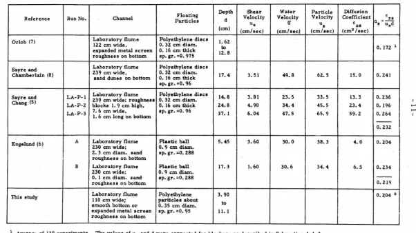
The average values of a. from each of the studies listed in Table 2. 2
s
range from O. 172 to 0. 241. They are less than the normalized
longitudinal coefficients given in Table 2. 1.
2. 2. 3. 2 Depth-Averaged Diffusion Coefficient. Because
Table 2. 2 Summary of published data on lateral diffusion of floating particles in open channels.
Depth Shear Water Particle Reference Run No. Channel Particles Floating d Velocity Velocity Velocity
u* ii' u
(cm) I
(cm/sec) (cm/aec) (cm/sec)
Orlob (7) Laboratory flume Polyethylene disc• l. 62 122 cm wide, 0. 32 cm diam.
to expanded metal screen 0. 16 cm thick
12.8 roughness on bottom ep. gr. =0. 975
Sayre and Laboratory flume Polyethylene discs
Chamberlain (8) 239 cm wide, O. 32 cm diam. 17.4 3. 51 49.8 62.5 sa_nd dunes on bottom O. 16 cm thick
ep.gr.=0.96
Sayre and LA-P-1 Laboratory flume Polyethylene discs 14. 8 3. 81 23.5 33.5 Chang (5) 239 cm wide; roughne11 0. 32 cm diam.
LA-P-2 blocks 1. 9 cm high,
·
o
:
16 cm thick 24.8 4.90 34.4 45. 5 LA-P-3 7. 6 cm wide, •P· gr. =O. 96 37. I 6.04 47.5 65. 9I. 6 cm long on bottom
Engelund (6) A Laboratory flume Plutic ball 5.45 3.60 30.0 38.3 230 cm wide; 0.9 cm diam.
2. 3 cm diam. sand ep.gr.=0.288 roughness on bottom
B Laboratory flume Plaetic ball 17.3 l. 60 30.6 34.4 230 cm wide; O. 9 cm diam.
O. l cm diam. sand ep.gr.=0.288 roughne u on bottom
Thie study Laboratory flume Polyethylene 3.90 110 cm wide; particlee about
smooth bottom or O. 35 cm diam. to expanded metal screen sp. gr. =O. 95 11. I roughness on bottom
1
Averag., o! lZO experiments. The values of u* and d were corrected for blockage as de1cribed in Subsection 4. l. 3. 3 Average o! 13 experiments. Data for all experimenta are given in Tables 4. 1 and 5. l.
Diffusion
Coefficient 'zs
E: ZI
a,=
u*d(cm3 /sec)
o. 172 1
15. 0 0.241
13. 3 0.236 23.4 o. 196 59.2 0.264
--
0. 2324.0 0.204
6.5 0.234
-0.219
-12-t. z , the depth-averaged value of the lateral turbulent diffusion . . coefficient. This coefficient is usually calculated with the formula
or
E:
z
where o2 is the variance of the lateral distribution of the depth-averaged concentration,
c,
and o~ is the variance of the lateral distribution ofac
I
az.
(2. lOa)
(2. lOb)
Eq. 2. lOa and b are obtained from Eq. 2. 3 as follows. Far
downstream from a source of a neutrally buoyant tracer, experimental data show that c' <<·c; therefore, one can delete each of the terms in Eq. 2. 3 that contain c' because there are corresponding similar terms containing
c.
One can also delete theterm~
aac
because it is less thanx x
a
-the deleted term
ax
(u'c' ). Therefore, for a steady source Eq. 2. 3becon1es
-
a-c
- a
2c-u -
ax
=
e: z8z2 - - · (2. 11)Taking moments of this expression in the z-direction yields Eq. 2. lOa, or taking the derivative of Eq. 2. 11 with respect to z and then taking
moments yields Eq. 2. lOb.
Values of
e
and the dimensionless coefficient ze
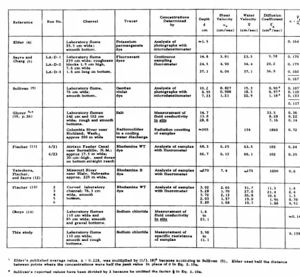
z Cl = Uo!<dfrom a number of investigations are given in Table 2. 3.
(2. 12)
These data can
-13-Table 2. 3 Sum1nary of published data on lateral diffusion of solutes in open channels.·
Elder (4)
Sayre a.nd
Ch&J?I (!>)
Sullivan (9)
Olover a,.•
110. p. 26)
Fi•cher ( 11)
Yatau.kura~
Flacher,
a.nd Sayre ( 12)
Fiecher (13)
Okoye (14)
Thi• etudy
Run No.
Laboratory flume
lS. 5 cm wide; amooth bottom.
Trac•r Pota•elum permanaan•k dye Concentration• D•t.rmlned by Depth d
Analyeh of ... 5 photo1raph• with
mlcrodanettomater
LA-D-1 Laboratory Ou.ma .Fluoreecent ContinUOlH
eamplin1
fiuororneter
14. 8 239 cm wide; rouahn••• dye•
L.A-D-2 block• 1. 9 cm hiah, 24. s
37. I 1. 6 cm wide
LA-D-3 I. 6 cm lona on bottom.
6/21 6/23
Laboratory fiwna,
76 cm wide; amooth bottom.
Analyeta of
pboto1raphe with
microd.enattometer
10.2 8. 9S 7. ]]
Laboratory Own•• Salt Meuureanent of fluid conducd vity
~~
14. 7
13. 8 28. 8 Z<&Z cm and IZZ cm
wide, rO\l&b and emootb
bottom•.
Colwnbla River near
Richland. Waeh.; approx 300 m wide
Radlonucllde• Radiation cou.ntin.1
ta a coolln1 of •ample•
water dlecbu1e
Atrl•co Fe9der Canal Rbodamlne WT Analy•t• of aample• 68. J
with tluorometer
near Bernalillo. N. M.; dye approx 17. S m widei
30-cm-hlah, •and dune•
on bottom atriU1ht reach
66. 7
Mbaourt River Rbodamlne B Analyeh of •amplti• ...270
with tluorometer
nea.r Blair, Nabruka dye a.pproa. ZZS m wide.
Curved laboratory Ahodaml.ne WT Analyete of •ample• 3. OZ channel: 76. l cm dye with tluorometer 5. 28
l. 72 2. 03 2. 20
wide, •mooth
bot:tnm.
La.bora.tory flwne•
110 cm 'fl'ida and
85 cm wt.de; unooth and 1ravel bottoma.
Laboratory tlume
110 cm wide;
•mooth and rou1h
bottom•.
Sodium chloride Meaaurecnent of
fluid conductivity
!!:!~
5odlwn chloride Mea•urement ol
apecillc re•latance
of aamplea
1.6
lo
21. I
l. 90
lo
11.l
Shear Water Oiffu•lon Velocity V•loclty Coeftlcient
u. u c.
(czn/••ol (cm/•ec) (cm• /••c)
3. 81 4. 90
6. 04
0. 827
o. 988
1.21
6. 29
6. 13
7.4
2. 66
1. 70
2. 13
I. )7
I. 68 23. s 34 ... 31. l
ts. 1
18. s
22. 9
134
63. s
66. I
... 11s
31. 7 27. 0
26. 8
19. 0 19. 7
9. SB
zo. 2 36. 9 0. 902 O. 97a
l. 182
H.S 8. 28 7. 16
1860
102 102
1200
11. 3
z I. ..
10.6
l. 96 I. 88
1
Eld•r1
• 1"-•hlhhiect Averaee vah.ae, o. ~ O. 228, waa multiplied by 0/1, ll)• becau•e A..:corJtn1 to 9.iWvan (9), Elder uaad half the diatance betw•en point• where &he concentration• ware h...U the pealt Yalue tn place of O tn Eq. 2. 10a.
• Su.lUyan'• report•d v&J1J•• hav• b••n divided by Z bec•u•• h• omitted the factor t ln i:.q. z. lOa.
~ Tr•cer• were not nautrall.f buoyant.
• Hydraulic radlue u•ed tn pl•c• of d•pth for compu.tin1 Q.
6 Averaae of 13 e.xperbnea.t•. Data for all ex:perim.ente are atvan in Table• '· 1 and S. 1.
o. 164 l
0. 170
o. 17'1
o. 160
0. 167
O. 107 a
0. 110 a
0. 133 2
0. 117 0. 36
o. 22
0. 14 o. 12
a. z4
0. ZS
0. 6
I. 4 2. 4
I. l
o. 70 0.1151
.. o. 14
-14-(Ref. 4, 5, 9, 10, 11, 14, this study) and the other from experiments in curved channels (Ref. 10, 12, 13). Except for the data by Glover, which were fron1 experin1ents in which the tracer was not neutrally buoyant, the data from straight channels yield values of
a
between O. 10 and 0. 25. (One should observe that the often quoted value published by Elder (4) has been corrected in Table 2. 3). All v a 1 u e s from curved ch an n e 1 s are greater than 0. 5. The higher values in curved channels have been explained by Fischer ( 13)as due to secondary currents induced by the bends. These currents transport material in the lateral direction by a process analogous to longitudinal dispersion as described in Subsection 2. 2. 1. Fischer was able to calculate a lateral dispersion coefficient using Eq. 2. 5 with lateral velocity deviations, w', in place of the longitudinal
velocity deviations, u 1 •
A suitable explanation for the variation in
a
for straight channels does not yet exist. However, it is worth noting that the range ina
found by one investigator is usually not as large as the range of the means of values given by different investigators. Therefore, much of the variation may be due to weak secondary currents characteristic
of the different flumes or channels. Attempts to correlate
a
to the width-to-depth ratio of the flow cross-section and to other parameters is presently being investigated by Okoye (14).In both the study by Sayre and Chang (5) and in this study, where
experiments were made to obtain both a and a , one finds that a is
s s
-15-the difference between a and as was sn1all if they used
u
in place of u in Eq. 2. 8, the data from this study do not confirm this re~;ult.s
2. 2. 4 Vertical Diffusion. An estimate of the vertical diffusion coefficient for mass in a wide open-channel flow, € , can be obtained
y
from the Reynolds analogy. One first expresses 'fxy' the apparent shear stress on a horizontal plane1 as
'f - (\ € )
au
xy - y y p
oy ,
(2. 13)where p is the fluid density, and the product A. € is the eddy viscosity. y y
The term
t.
is the turbulent Schmidt number and is the ratio of ythe diffusion coefficients for momentum to mass. Using the Prandtl-von Karman logarithmic velocity distribution,
u
,:c
u(y) - u(d)
=
k
tn~, (2. 14)and a linear distribution of shear stress,
(2. 15)
Eq. 2. 13 yields
(2. 16)
This expression for A. t. is zero at y
=
0 and y = d, and is symmetric y yd
about y
=z
·
The depth-averaged value is given by k\yey
=
6
u*d . (2. 17)Vanoni ( 15) observed the vertical distributions of suspended sedi-ment in an open-channel flow and.used the data to calculate e for ·sediment.
y
-16-and that A ~ 1. Jobson and Sayre (16) introduced dye at the surface
y
of an open-channel flow and observed the vertical distributions of
dye as a function of distance downstream. They used the data to
calculate i:: and also found that E: and A E: were sirnilarly distributed
y y y y
and that >.. :-"'3 1. Similar experiments with fine sediment gave nearly
y
1 '1<' t;;11111· result!~.
/... 1 1~:Ft•'l•~CTS OF DENSITY DIFFEHENCES ON MASS THANSFEH
2. 3. 1 Vertical Density Gradients. Observations of vertical
tur-bulent diffusion in the atmosphere, in natural water bodies, and in the
laboratory show that stable vertical density gradients reduce vertical
diffusion (Ref. 17 and 18). Observations also show that the
vertical diffusion of mass or heat is reduced more than the diffusion
of momentum. Taylor ( 19) noticed that stable density gradients in
the atnwsphere reduce turbulent wind velocity fluctuations in all three
dir.ect:iom;; hence, one n1ay suspect that a stable vertical density
).;.radil.'nt. J1"1ay r1.~d11c<· turb1d.cnt diffui,;ion in the hori.zontal direction
also.
Ellison and Turner ( 18) have given a physical explanation for the
reduction in vertical diffusion by a stable density gradient. They
reasoned that a parcel of fluid which is displaced from its equilibrium
postition by turbulence m ay return to its equilibrium position before
it mixes completely with the surrounding fluid. They also reason that
the reduction in the diffusion of momentum is not as great as the
-17-exchange m01nentum without .mixing by the action of pressure, but jn order to transfer heat or mass the parcel of fluid must mix with its
surroundings.
Most investigators attempt to relate the decrease in diffusion caused by a stable density gradient to Ri, the Richardson number,
Ri
=
g_
~
/ (
au)a
p
Hy
Cly ' (2. 18)whcrv !-'. is the ~cceleration due to gravity, and 8u/()y lA the vertical gradient of the primary flow which is considered to be horizontal. Munk and Anderson (17) suggest the empirical equations:
e A.
=
(e A. )0 (l +Ri)-ty y y y (2. l 9)
and
e
=
(e )o (1+130Ri)-~,
y
y
(2. 20)where (e: y )., y )0 and (t. y )0 are the values of
e
y y A. ande
y under neutral conditions, Ri -= 0. Okubo (20) reviews formulae suggested by otheri.1 tVf' H tig;ttnr H.
Because the longitudinal dispersion coefficient, D , given by x
Eq. 2. 5 is inversely proportional to
e
,
one may expect that D wouldy
.
xbe larger for stable density-stratified flows than for flows of uniform density.
2. 3. 2 Horizontal Density Gradients. Observations show that density differences in the horizontal direction can increase mass
-18-homogeneous turbulent field. They found that the rate of mixing of the two fluids increased with increasing density difference. Jen, Wiegel,
and Mobarek (22) and Hayashi and Shuto (23) performed experiments with heated jets of water that discharged horizontally near a free
surface; they found that lateral spreading of the jets increased with increasing difference in temperature between the discharged and ambient fluids.
Density-induced velocities also occur in estuaries, where long i-tudinal density gradients exist due to the difference in density between salt water frorn the ocean and fresh water from rivers. Experiments in an idealized laboratory estuary by Ippen, Harleman, and Lin (2 ),
which are analysed and are described in more detail in Chapter 6, show that as the difference in density between the water in the ocean and
incoming river increases, the apparent longitudinal diffusion coefficient increases also. Ippen (24) has explained conceptually the effect of
longitudinal density gradients on the velocity distributions in estuaries, and Hansen and Rattray (25) have treated the problem analytically. If
the pressure distribution over the vertical is hydrostatic, and if the
estuary is well nlixcd vertically so that the variation in density with depth is small, the pressure is given by
p
=
(d-y) pg.If the x-axis is horizontal, the longitudinal pressure gradient is then
given by
(y-d) g *
+
Spg =- .££
ax , (2. 21)
-19-vertical distribution of each of the terms in Eq. 2. 21 are shown in Fig. 2. 1 for a seaward sloping water surface. Because the pressure gradient due to the water surface slope is invariant with depth, and because the pressure gradient due to the density gradient is zero at the water surface and reaches a maximum at the botto1n, the resultant pressure gradient near the surface and near the bottom can be in opposite directions. The result can be an upstream flow near the
bottom but a downstream flow near the surface. When used in Eq. 2. 5, velocity distributions of this type yield higher longitudinal diffusion coefficients than unidirectional velocity distributions with the same xnean velocity. Because the upstream flow in the lower layer must
return seaward in the upper layer, the flow pattern resembles a longitudinal circulation of the primary flow.
The present study investigates the effects of density-induced secondary circulation on lateral mixing in turbulent open-channel flows with lateral density gradients.
y
ap
(y-d) g
ax
+
Spg
=
"""
\
'
. ./
-20-CHAPTER 3
EXPERIMENTAL APPARATUS AND TECHNIQUES
3. 1 DESCRIPTION OF EXPERIMENTS
Experiments were n1ade in a laboratory flume to observe the
lateral mixing of fluids with densities different from that of the
ambient flow. The objective of the experiments was to obtain data
for developing and checking techniques for predicting horizontal
mixing rates in turbulent flows with horizontal density gradients.
In the experiments, a tracer fluid was introduced continuously
into the flume uniformly over the depth and across some fraction
of the flume width. The tracer fluid was introduced into the flume at
the same velocity as the ambient flow in the flume. In most
experiments, the source was located on the flume center line, and the width of the source was small compared with the width of the flume.
However, in some experiments that were made to observe the
mixing of two wide parallel streams, the tracer fluid inihally occupied all that part of the cross -section on one side of the flume center line.
Most experiments were made with tracer fluids whose densities
were slightly greater or the same as the density of the ambient water
-21-fluids which were less dense than th() ambient water. All tracer
fluids were salt water (NaCl) solutions. The densities of the heavy
tracer fluids were varied by changing the salt concentrations. Tracer
fluids of neutral density were prepared by adding methyl alcohol to
a salt-water solution. The light tracer fluids were made by adding
additional amounts of alcohol. The tracer fluids were often colored
with an organic dye to make them visible.
Distributions of tracer fluid in cross -sections downstream from
a source were obtained by taking water samples from points in the
cross- sections and by measuring the specific electrical resista~ce
of each sample to determine the tracer concentration in each sample.
The lateral diffusion of small floats was observed during
experi-ments in which the tracer fluid was neutrally buoyant and also in
experiments in which no tracer fluid was introduced into the flume.
The purpose of these experiments was to provide additional data to
compare the turbulent diffusing characteristics of the flows in the
flumes used in this study with the flows in the flumes used by other
investigators.
3. 2 FLUME
3. 2. 1 Description. The experiments were conducted in a
40-meter-long recirculating flume located in the sub-basement of the
W. M. Keck Laboratory of Hydraulics and Water Resources.
Fabrication details of the flume are given by Vanoni, Brooks, and
.,
-..
.,..
,
,
,
"
.
..
'·~'--- . I
'·
0 ; ! I 110.0 cm (INSIDE)
[1
- r--- -- ---1
I
I
I -tl- ~f- '11 I; l•r = =9 I . •: .
. I I !•
; Ci ~' r----_J " ! ;
I
I !! ~ J ' . ! _____;.-
; )}
' :· ·;
,.
i 1L ___ - - --- _j ._ _ _ .J ---,~-'
WEIR__/ . ~ .:
!._ - - --- - - -- - - --- ---- 38.57m - -- -- - -- - - -- -, ~---R-E=OtR ::::::.7---_-_-:_-_-_-:_-:_-_-;.-;_"0--:-_-:_-:_~·-;
- INLET TANK
STAINLESS STEEL
-PLATE
f SCREEN SECTION
1- STAINLESS STEEL
i SIDES
-,:'W </
\
i RllBSER. PIPE \_JACK
SECTION A-A ENLARGED X3
A
VENTURI METERS .
i i - 3.007m- , ---· -·-49 a534m--- -·---1
GLASS SIDES ~.
\
/. . .t". / j ,;~/-~/
L JACIC DRIVE SHAFT
- - -- - - --- - - -- ---- - - -- -· 4084m- - -- - - I
STAINLESS STEEL SIDES-,
\
' I
RESERVOIRS"?>.,.
! , ..
OUTLET-,
TAM<
!
I
r -3£96m-
-·
..
·
...NOTE: ARROWS---DENOTE FLOW PATH
Figure 3. 1 The 40-meter flume. (Drawing modified from Vanoni et al. (26) ).
I N
-23-in the photograph in Fig. 3. 7. The bottom of the flume is made of stainless steel plate and is 110 cm wide; the vertical sidewalls arc
(il cn1 high and are glass alollg most of the flunw's length. An instrument carriage rides on rails which are n10unted on the tops of the sidewalls.
The flume is supported in pivot bearings near its mid-point and is supported elsewhere by four pairs of power-driven screw jacks
(as shown in Fig. 3. 1 ). The flume slope is obtained by reading a vertical staff attached to the flume approximately 17 meters upstream from the pivot. The staff was calibrated by observing the slope of
the flume bottom with respect to a still water level.
3. 2. 2 Water Circulation. Water entered the upstream end of the flume through a metal screen (8 mesh/ inch) from a baffled inlet tank. An adjustable weir was installed at the downstream end of the flume to control the tail-water depth. Water flowed over the weir into an outlet tank.
The design of the flume permits a number of alternatives for returning the water fron1 the outlet tank to the inlet tank. In order to n1inimize changes in the tracer concentration of the ambient
flow during an experiment, the return system was modified to utilize the maximum water volume. Water flowed from the outlet
tank through a pipe and a laboratory floor drain into the farthest of the four reservoirs. The reservoirs are connected in series by short lengths of 10-inch pipes. The reservoirs have a combined
-24-frorn the last reservoir, which is under the outlet tank, through a nominal 8-inch pipe, which runs under the flume, to the inlet tank.
The pump was driven by a IO-horsepower motor through a contin-uously variable V-belt drive. Water discharge was measured with
a venturi meter (Keck Lab. No. Q-6) in the 8-inch pipe. The 16-inch pipe which runs beneath the flume was not used for the return flow and was capped near the outlet tank but was allowed to fill with water from the inlet tank.
3. 2. 3 Rough Bottom. The bottom of the flume was made rough for s01ne experiments by laying expanded metal sheets (Fig. 3. 2) on
the stainless steel bottom. The sheets, which are manufactured for use as plastering lath, are made of steel and are galvanized; their approximate dimensions are given in Fig. 3. 3. Although the total thickness of the lath is 0.31 cm,the solid volume is equivalent to that of a solid sheet only 0. 025 cm thick.
The lath was cut into panels 73 cm by 109 cm which were installed with the 109 cm length spanning the width of the flume.
The panels were held to the stainless steel botom with mastic stripping 1 /2 inches wide by 1 /8 inches thick. Single strips of mastic were laid about 5 cm from each wall along the entire length of the flun1.e, and three pieces about 8 cm long were laid longitudin-ally at the joints between panels. The panels were pressed into the mastic so that they lay flat on the stainless steel bottom.
-25-· flow direction
scale reads in centimeters IJll/ !l,1111/llll/Jllljlllllllllllllllllll\llll\llll\111111111\ll\1\llll\1111\ I
6 7 8 9 10 l l 12 13
1 0 1 1 6
Figure 3. 2 Photograph of expanded metal lath used for roughness on the bottom of the flume.
O.Blcm
E
g
~ ~.,,
"-~r
m fouumed bottom stoinleu steel bottom
SECTION A-A
Figure 3. 3 Dimensioned sketch of metal lath used for
-26-3. 3 WATER DEPTH AND VELOCITY MEASURING EQUIPMENT
Water depths in the fluine were measured with a point gage
which could be read to the ncarcHt 0. 01 ctn and which waH rnountt-~cr
on the instrurnent carriage.
Water velocities were measured with a 1 /8 inch (0. 32-cm)
diameter pitot- static tube. The differences in pressure between
the dynamic and static ports were measured electronically with
a pressure transducer and strip-chart recorder. The system was
calibrated by imposing pressures on the transducer with a water
manometer which could be read to within O. 001 inches (0. 0025 cm).
The difference between calibrations before and after an experiment
was always less than two percent.
The pitot-static tube was attached to the traveler of a point
gage on the instrument carriage for positioning it in the flume. To
obtain the velocity at a point,the output of the pres sure transducer
was recorded for 30 seconds and was averaged by eye.
3. 4 TRACER FLUID SYSTEM
3. 4. 1 Fluid Handling System. The tracer fluids were prepared
in a mixing tank and were pumped into the flume through various
types of sources which are described in Section 3. 4. 2. The mixing
tank was open at the top and had a capacity of approximately 600 liters.
The tank and associated plumbing are shown schematically in Fig. 3. 4.
The mixing tank was filled with water from the 16-inch
SHUTOFF
VALVE
I I ~ YZ . . . -~---i'O'...----~
TO SOURCE
REGULATING )If
VALVE
I
IN FLUME
VALVE
PUMP
FLOOR
I
I
01
I
FLOWMETER
t
•
I
I
VALVES
MIXING
TANK
· - - 4-•yx=i. n
- - - . . _ , ~JS'Sll ,5,;p
·. ··:<:>:
~··.
:~.:·:
·:.~:-.: :·:·!>.::~.:: :.~.":. :·~:~.Jr
:
:
j;:
A··
.
-:
·
·
..
:.-::·~:-
:.::
'
...
~:A"·:.:4;-.;~ ~;:
o
.
~.·,.A . •·.'!'
.
•
•
..
.o .. -.~.·.A.·.
.•..
.
.. ·
.
· .. ,
~·.:.
..
~-.
...
·
.·
..
·
.
. · ,
.
I
..---
--
---i'
1---....,..
16- INCH PIPE
Figure 3. 4 Schematic drawing of the tracer-fluid handling system.
,
-28-alcohol (if any) were added to the tank and were mixed by pumping water out of the bottom of the tank and returning it at the top.
For soni.e experiments dye was also added to the solution.
During most experiments, fluid was pumped from the rnixing tank to the source in the flume. However, for some experiments, wat·er with no tracer and with the sam e density as the flu.id in the
flt11.111· w:IN p1111q>1:d din •c.,'.Ll.y ft•t1nl tlu· J(, .. inch pip1~ l.o I.hi: 1-101n·cc.
Tht~ .r.low rate tn tlie source was ineasured with a variable area
flown1eter (Keck Lab. No. Q-29) and was regulated with a gate
valve. A shutoff ball valve was put in series with the regulating valve for convenience.
3. 4. 2. Sources. The tracer sources in the flume were designed
to distribute the tracer uniformly over the depth and across some
selected width within the flume. They were also designed to cause rninimun1 disturbances to the ambient flow. Three designs were
11:-;ed: 011c design was used for the narrow sources, cm and 2 cm ,vidc; a second design was used for the 12. 5-cm - and 20-cm-wide i.nternicdiate width sonrces; and the third design was used for the
wide source in which the tracer was distributed over one-half of
the 110-cm-wide flume.
3. 4. 2. 1 Narrow Sources. The narrow I-cm-wide source, which is shown in Fig. 3. 5, was made by placing a vertical manifold between two vertical guide walls. The manifold was a
flath med length of thin-walled brass tubing with holes drilled in
-29-1 OT09.
Figure 3. 5 The 1-cm-wide source.
10114
-30-0. 3 cn1. intervals along a vertical line starting near the botto1n and
extending about 11 cm high. Holes above the water surface were cove:r.ed with plastic tapE:~. The holes were 1nadf'. with a l /8-inch
-di;U.))1::t,•1.· drill and overy th'i1·rl hole: w;ui t•nl;1rged t:o a J/1(1-
inch-di.:irnch'r. A µiece of rolled wire screen was placed in front of the manifold to break up the jets from the manifold.
The vertical guide walls were made of 24-gage (0. 028-inch)
galvani:;,ed steel sheet. They were 1 cm apart and parallel at the
downstrea1n end but met to form a sharp edge at the upstream end.
The total length of this source was 25 cm. The surface waves generated by this shape were less than 0. 15 cm high and were not
much larger than the waves 1nade by a single piece of sheet metal
placed parallel to the flow.
The di::;cha.rge fron1 the 1-crn-wicle source was equal to the
dischar~e through a l-cn1-wide vertical strip in the central part
of the flltmc. The velocity distribution at the mouth of the source was oh8erved to be approxim.atcly uniform over the depth. The downstream end of this source was located 15 meters downstream
from the screen in the inlet box of the flume.
A 2-cm-wide source, 61 cm long, was constructed similar to
the I-cm-wide source. However, the 2-cm-wide source was·us.ed
only in an experiment to observe the lateral diffusion of floating
-31-3. 4. 2. 2 The Intermediate Width Sources. The 12. 5-crn-·
and 20 -crn-wide sources were n1adc by placing a horizontal manifold between two parallel vertical guide walls. The guide walls were open at each end to allow the watc:~r in the flunw to flow l.rntwec n then1. A tracer fluid fron1 the mixing tank was sprayecl by the inanifold onto the surface of the water flowing between the guide walls. This design did not require mixing, storing, and pumping large volumes of water as would be required if the sources were constructed in the same way as the narrow sources. The 20-cm-wide source is shown in Fig. 3. 6.
The sa1ne guide walls were used for both sources. They were 9 J.,5 crn long, 20. 3 cm high, and were made from 18- gage (0. 049-inch) stainless steel sheet. The walls were fastened to metal rods of the proper length which held them apart and upright. The contact between the guide walls and the rough lath bottom was sealed with mastic. Plastic tape was used to seal the contact between the guide walls and the smooth bottom.
-32-cross-piece. The holes were spaced 1. 25 cn1 apart in lhe nianifol<l
for the 20-cni-wide source, and 0. 65 cn1 apart in the 1nanifold. for
the 12. 5-cin-wide source. The holes were approximately O. 25 crn
in diarnt•tcr; thl~ holes were niadc sli1i;htJy larger nc<.1r !:he ct•ntc:r
a1HJ s1nalh'!r 11<::.n· the C'nd ~; i.n ord<~r t.o 1nake the tracer concn11tratio11
distribution n1ore nearly uniforin across the source.
Flow rates through these manifolds were the same or less than
the flow rates through the manifold in the narrow I-cm-wide
source. The combination of these flow rates and manifold port
sizes produced jets which penetrated the water to give sufficient
rnixing over the depth but did not excessively disturb the flow. The
manifolds were tilted slightly to give the jets a small downstream
con1ponent of rr\01nentun1 to oppose the hydraulic resistance of the
~uide waUs on the flow between them. The downstrean1. ends of the .
gltide walls for both these sources were ] 7. 8 n1eters downstrean1
fron1 the screen in the inlet box.
Almost all experiments with the 1-cm-, 12. 5-cm-, and 20-c
m-wide sources were conducted with the sources on the center line of
the flume. To test the applicability of the data from the experiments
to proble1ns in which an effluent is discharged along the bank of a
stream, a 10-crn-wide source was placed against the left sidewall
of the flun1e. Data fro1n experiments with this source were analysed
as if the wall were a line of symmetry for the 20-cm-wide source.
-33
-111 lhl):.;c 11~:c:d i.:1 lhc ll.. r;_ ,·n1 · .11H] /.O·cl1.1··wjd,· :-:11111·1·1•1·:, l11d: 'Jtllll)!. unly Pti.· ~·.11id1~ w .. \.11, wllil·l1 w.-H• placed JO 1·111 .1'1·11111 tl1t• :'1id.·wa..ll
oJ the .f Jn 1 nc.
3. 1. 2. 3 Wicl~' Source. The widest source used i11 the
c.xperi.n1ents occupied half the width of the 110-crn -wide fhune.
This source was used to study mixing of two wide parallel streams of the sa1ne depth and flowing with the same velocity but having
different concentrations or densities. This wide source, shown
in Fig. 3. 7, was made by partitioning the flume along part of its l1·11µ;th wit.h a longitudinal di vidi.ng wall and spraying a tracer into
<llh' :3lcl1· <Jf t.IJ<• flu1nc. nc·c-a111:1e of the 1:1y·nnnc•t:ry of t111~ apparat:ui:;.
on1• can observe sin1.ultaneously ir1 one experi.n1ent th.e rnixing of a heavy fluid into a light one, and a light fluid into a heavy one.
The dividing wall was 7. 3 meters long and 20 cm high. The
upstream end was 5. 3 meters downstream from the screen in the
inlet box of the flume. The wall was made from three pieces of 18-gage
(0. 049-inch) galvanized steel sheet which were put end to end. Each
sheet was stiffened by bending the top at a right angle to form a
narrow flange. The wall was laterally braced every 60 cm by
wcdgii1g wooden st:rnts between the wall and th<~ sides of the flume.
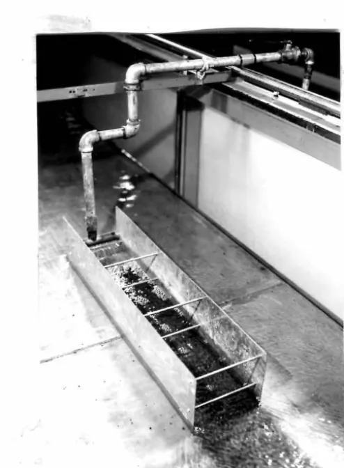
10048
Figure 3. 7 Photograph looking down the flume.
The splitter wall for the wide source is in the center, and the manifold is on the left.
:.,,J ..:.
~ ~ :J 3~
-35-The tracer fluid was sprayed from a n1anifolc1 into the flunie
on the lefl side (looking clownstrea1n) of t:h