University of Windsor University of Windsor
Scholarship at UWindsor
Scholarship at UWindsor
Electronic Theses and Dissertations Theses, Dissertations, and Major Papers
2009
Turbulent structures in smooth and rough open channel flows:
Turbulent structures in smooth and rough open channel flows:
effect of depth
effect of depth
Vesselina Roussinova University of Windsor
Follow this and additional works at: https://scholar.uwindsor.ca/etd
Recommended Citation Recommended Citation
Roussinova, Vesselina, "Turbulent structures in smooth and rough open channel flows: effect of depth" (2009). Electronic Theses and Dissertations. 94.
https://scholar.uwindsor.ca/etd/94
Turbulent structures in smooth and rough open channel flows: effect of depth
by
Vesselina Tzvetanova Roussinova
A Dissertation
Submitted to the Faculty of Graduate Studies through Civil and Environmental Engineering
in Partial Fulfillment of the Requirements for the Degree of Doctor of Philosophy at the
University of Windsor
Windsor, Ontario, Canada
2009
DECLARATION OF CO-AUTHORSHIP\PREVIOUS PUBLICATIONS
I. Co-Authorship Declaration
I hereby declare that this thesis incorporates material that is result of joint research, as follows:
This thesis also incorporates the outcome of a joint research undertaken in collaboration with Vesselina Roussinova under the supervision of professors Ram Balachandar and Nihar Biswas. The collaboration is covered in Chapters 2, 3, 4 and 5 of the thesis. In all cases, the key ideas, primary contributions, experimental designs, data analysis and interpretation, were performed by the author, and the contribution of co-authors was primarily through the provision of supervision
I am aware of the University of Windsor Senate Policy on Authorship and I certify that I have properly acknowledged the contribution of other researchers to my thesis, and have obtained written permission from each of the co-author(s) to include the above material(s) in my thesis.
I certify that, with the above qualification, this thesis, and the research to which it refers, is the product of my own work.
II. Declaration of Previous Publication
This thesis includes 4 original papers that have been previously published/submitted for publication in peer reviewed journals, as follows:
Thesis Chapter Publication title/full citation Publication status
Chapter 3
Roussinova, V., Biswas, N., and Balachandar, R. (2008). “Revisiting turbulence in smooth uniform open channel flow.” J. Hydr. Res., 46, 1, 36-48.
published
Chapter 4
Roussinova, V., Shinneeb A.-M. and
Balachandar R. (2008) “Investigation of fluid structures in a smooth open channel flow using proper orthogonal decomposition (POD)” J.
Hydr. Engrg.
under review
Chapter 5 Roussinova, V., and Balachandar R. (2008) “Effect of depth on flow past a train of rib elements in an open channel” J. Hyd. Engrg.
under review
Chapters 3 and 5
Roussinova, V., Biswas, N., and Balachandar, R. (2009) “Reynolds stress anisotropy in open channel flow.” J. Hydr. Engrg.
I certify that I have obtained a written permission from the copyright owner(s) to include the above published material(s) in my thesis. I certify that the above material describes work completed during my registration as graduate student at the University of Windsor.
I declare that, to the best of my knowledge, my thesis does not infringe upon anyone’s copyright nor violate any proprietary rights and that any ideas, techniques, quotations, or any other material from the work of other people included in my thesis, published or otherwise, are fully acknowledged in accordance with the standard referencing practices. Furthermore, to the extent that I have included copyrighted material that surpasses the bounds of fair dealing within the meaning of the Canada Copyright Act, I certify that I have obtained a written permission from the copyright owner(s) to include such material(s) in my thesis.
I declare that this is a true copy of my thesis, including any final revisions, as approved by my thesis committee and the Graduate Studies office, and that this thesis has not been submitted for a higher degree to any other University or Institution
ABSTRACT
In this thesis, detailed experiments are performed to study the effect of the flow depth
on turbulent structures in smooth and rough bed open channel flow. Shallow open
channel flow is dominated entirely by the wall turbulence with a wall boundary layer that
occupies a significant fraction of the flow depth. When the rough bed is introduced in the
shallow flow, the local turbulence near the roughness element intensifies and becomes
highly heterogeneous. The model roughness under study consists of a train of two
dimensional square ribs spanning the whole length of the channel. The height of the ribs
(k) occupy 10-15% of the depth of flow (d) and falls in the category of large roughness.
The experimental program was designed to study k-and d-type roughnesses at
intermediate flow submergence (6 < d/k < 10). Velocity measurements were conducted
using laser Doppler velocimetry (LDV) and particle image velocimetry (PIV) systems.
While on the smooth bed, mean velocity scaling in the classical logarithmic format
was confirmed from the present experiments, for the deep-flow cases, turbulence
quantities were found to be influenced by the free surface. A modified length scale based
on a region of constant turbulence intensity is proposed to account for the effect of the
free surface. The new length scale provides a better description not only for the mean
velocity profiles but also for the Reynolds shear stress profiles and correlation
coefficients. With the use of this new length scale, the estimation of the wake parameter
is positive and provides for a more accurate estimate of the friction velocity.
Two-dimensional PIV measurements were made in the streamwise-wall normal plane
of the smooth open channel flow at d = 0.10 m and Red = 21,000 (Red = dU0/
ν
) toorthogonal decomposition (POD) and swirling strength analysis were employed to
investigate the structures present in the flow. Analysis of the POD reconstructed velocity
fields reveals the presence of large-scale energetic structures near the free surface. These
structures are almost parallel or slightly inclined to the free surface creating long zones
with uniform momentum.
When large distributed bed roughness is introduced in the open channel, the
anisotropy of the Reynolds stresses is reduced in the outer layer and found to depend on
the rib spacing and roughness density. At shallow depth, the presence of roughness
increases the turbulence intensities, Reynolds shear stress and higher-order moments in
the outer layer of various locations along the rib wavelength. While for the shallow
depth, the ratio of the shear contribution of sweep to ejection events is very different from
that obtained on the smooth bed, for the deep flow cases, this difference diminishes in the
DEDICATION
ACKNOWLEDGEMENTS
Many people contributed to this work and made it possible. I would like first to
sincerely thank my advisors Dr. Ram Balachandar and Dr. Nihar Biswas for their
inspiration, guidance and support during my PhD study at the University of Windsor.
I would also like to thank all of my colleagues Faruque, Arindam and Arjun with
whom I shared an office for the last 5 years. Their curiosity and helpful discussions
provided an enriching environment to work in.
Many thanks also go to Dr. Stefano Leonardi of the University of Puerto
Rico-Mayagüez for making his DNS simulation on rough wall available to me.
I would like also to acknowledge the encouragement and support received from my
family especially from my husband without him this work could not have been possible.
Finally, this work was made it possible by the financial support of the National
Science and Engineering Research of Canada (NSERC) through Canadian Graduate
TABLE OF CONTENTS
DECLARATION OF CO-AUTHORSHIP\PREVIOUS PUBLICATIONS ... iii
ABSTRACT...v
DEDICATION... vii
ACKNOWLEDGEMENTS... viii
LIST OF TABLES ... xi
LIST OF FIGURES ... xii
LIST OF SYMBOLS ... xviii
I. INTRODUCTION 1.1. Motivation ...1
1.2. Background ...4
1.2.1.Turbulent boundary layers vs. open channel flows ...5
1.2.2.Shallow open channel flow...13
1.2.3.Rough open channel flow ...15
1.3. Research objectives and thesis overview ...22
II. EXPERIMENTS 2.1. Open channel flume facilities ...26
2.2. Velocity measurements ...29
2.2.1.Laser Doppler velocimetry (LDV) ...29
2.2.2.Particle image velocimetry (PIV) ...30
III. TURBULENCE IN SMOOTH UNIFORM OPEN CHANNEL FLOW 3.1. Mean velocity scaling and friction velocity ...39
3.2. Turbulence intensities ...44
3.3. Higher order moments ...45
3.4. Conditional quadrant analysis ...46
3.5. Anisotropy analysis...51
3.5.1.Correlation coefficient ...52
3.5.2.Reynolds stress anisotropy analysis...53
IV. TURBULENT STRUCTURES IN SMOOTH OPEN CHANNEL FLOW
4.1. Proper Orthogonal Decomposition (POD)...70
4.1.1.Theory...71
4.1.2.POD analysis of smooth open channel flow at (x-y) plane....75
4.1.3.Vortex visualization and statistics ...80
4.2. Zones of the uniform momentum...84
4.3. Conditional quadrant PIV analysis ...89
4.4. Summary ...94
V. EFFECT OF DEPTH ON FLOW PAST A TRAIN OF LARGE RIB ELEMENTS IN AN OPEN CHANNEL 5.1. Mean velocity profiles...111
5.2. Turbulence intensities and Reynolds shear stress ...116
5.3. Conditional quadrant analysis ...120
5.4. Anisotropy analysis...127
5.4.1.Effect of the p/k at constant flow depth d = 0.1 m ...128
5.4.2.Effect of the flow depth ...132
5.5. Summary ...134
VI. CONCLUSIONS, CONTRIBUTIONS AND FURURE RECOMENDATIONS 6.1. Smooth open channel flow...153
6.2. Rough open channel flow...157
6.3. Future work ...159
VII. REFERENCES APPENDIX A UNCERTAINTY ESTIMATES AND VELOCITY VALIDATION A.1. LDV measurements...172
A.2. PIV measurements ...178
A.3. PIV validation ...179
LIST OF TABLES
Table II-1. Experimental conditions for the smooth OCF experiments... 32
Table II-2. Experimental conditions for the rough OCF tests ... 32
Table III-1. Calculated friction velocities... 58
Table III-2. New defect law parameters (Krogstad et al., 1992) calculated with a
modified length scale δ′. ... 58
Table A-1 Typical uncertainty estimates for smooth and rough OCF at y/d = 0.5... 177
LIST OF FIGURES
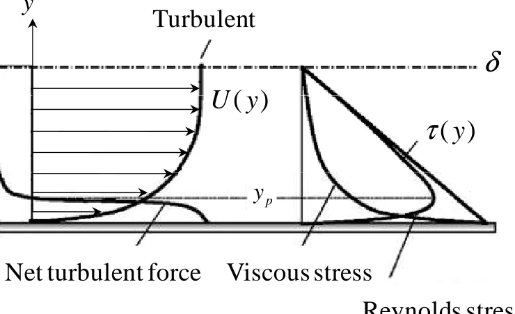
Figure I-1. Velocity profile and variations of Reynolds shear stress and viscous stress in
a turbulent channel flow... 24
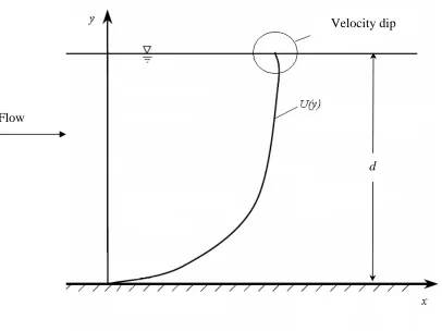
Figure I-2. Velocity profile of uniform smooth open channel flow. ... 25
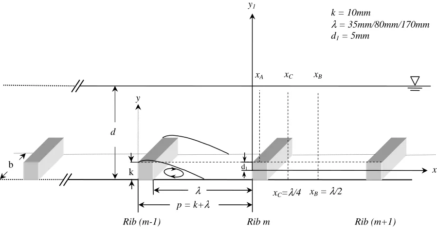
Figure II-1. Turbulent flow over a train of ribs (not to scale)... 33
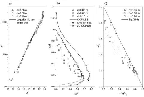
Figure III-1. Determination of the uτ for smooth OCF; a) Log-law format b) Classical
scaling for the Reynolds shear stress profiles and c) Total shear stress distributions. 1
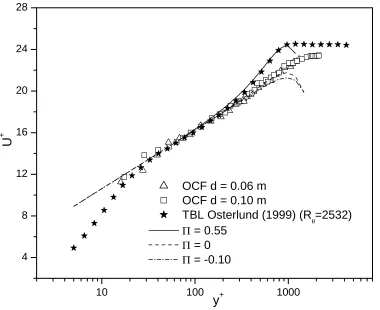
Figure III-2. Velocity defect profiles in inner scaling. Comparison between the wake
functions proposed by Coles (1956) (Eq. (III.7)) and Krogstad et al., (1992) (Eq.
(III.8)... 1
Figure III-3. Outer scaling of the turbulent intensities showing a subsurface region of
constant turbulent intensity for d = 0.06 m, 0.08 m and 0.10 m. ... 1
Figure III-4. Improved outer region scaling for various turbulence quantities. Legend as
in Figure III-1... 62
Figure III-5. Inner (a and b) and outer scaling (c and d) of the longitudinal (Du) and
vertical (Dv) turbulent fluxes of shear stress. Symbols as in Figure III-1. ... 1
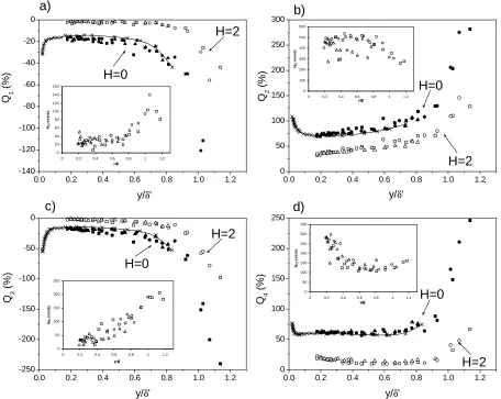
Figure III-6. Comparison between open channel flow and turbulent boundary layer data
by Schultz et al., (2005) at H=0 (a) Q2 and (b) Q4 and at H=2 (c) Q2 and (d) Q4.
Symbols as in Figure III-1. ... 1
Figure III-7. Comparison between open channel flow and 2-D channel data by Krogstad
Figure III-8. Distributions of the third order moments (u3+ ) in open channel flow, turbulent boundary layer (Schultz et al., 2005) and two-dimensional channel
(Bakken et al., 2005a). Symbols as in Figure III-1... 1
Figure III-9. Ratio between Q2 and Q4 contributions in outer variables at H = 0 and H =
2.5 of open channel flow and two-dimensional channel (Bakken et al., 2001).
Symbols as in Figure III-1. ... 1
Figure III-10. Coefficients of correlation,
ρ
uv for the smooth open channel flow at threedifferent flow depths of d = 0.06 m, 0.08 m and 0.10 m. Improved scaling is shown
in (b)... 1
Figure III-11. Components of the bij for the smooth open channel flow at three different
flow depths 0.06 m, 0.08 m and 0.10 m. Solid lines denote the DNS simulations of
Leonardi et al., (2006) on the smooth wall while dash lines denote the free surface
simulations of Handler et al., (1993). ... 1
Figure IV-1. Velocity fields of smooth OCF at d = 0.10 m a) mean velocity field from
2000 images, b) instantaneous velocity field at t = 17.3 s and c) instantaneous
velocity field at t = 28.1 s. The mean flow direction is from left to right... 1
Figure IV-2. POD energy distributions of the smooth open channel flow in the (x-y)
palne. Fractional (solid symbols) contribution of each POD mode and cumulative
(open symbols) distribution. ... 1
Figure IV-3. Examples of a) a fluctuating velocity field, and b), c), and d)
POD-reconstructed fluctuating velocity fields using the first 12 modes. These modes
recovered 50% of the turbulent kinetic energy. Note that only every second vector
Figure IV-4. Two examples a) and b) of POD-reconstructed fluctuating velocity fields
using modes 13 to 100. These modes recovered about 33% of the turbulent kinetic
energy. Dark and light grey circles represent positive and negative rotational sense,
respectively. ... 101
Figure IV-5. Example of the fluctuating velocity field in the (x-y)-plane with positive
(retrograde) swirl (red shading) and negative (prograde) swirl (blue shading)
superimposed. ... 102
Figure IV-6. Statistics of the swirling strength in the (x-y) plane showing the fraction of
time with positive(Tλ+), negative (Tλ-) and non-zero (Tλ≠0) swirling strength... 103
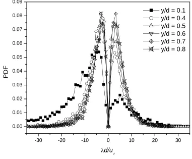
Figure IV-7. Probability density functions of the dimensionless swirling strength in the
(x-y) plane at different wall-normal locations. ... 104
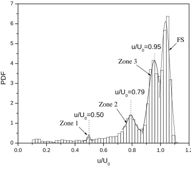
Figure IV-8. Histogram of the relative distribution of the instantaneous velocity field at t
= 17.3 s showing the zones of the uniform momentum... 105
Figure IV-9. Vortices along the boundaries of the uniform-momentum zones. The
vortices are identified with the swirling strength. The black lines separate the flow
field into zones, labelled 1, 2 and 3 in which the streamwise momentum is nearly
uniform. Instantaneous velocity vector map (t = 17.3 s) in a convection frame of
reference Uc = 0.95U0 is also shown... 106
Figure IV-10. Zones of streamwise uniform momentum of the two velocity fields a) at t
= 17.3 s and b) t = 28.1 s. The color map corresponds to (u−U0)/uτ, where U0 is
time-averaged, maximum velocity and uτ is the friction velocity. ... 1
Figure IV-11. Color maps representing the quadrant analysis of instantaneous fluctuating
Figure IV-12. Color maps representing the quadrant analysis of instantaneous fluctuating
velocity field shown in Figure IV-1c a) H = 0, b) H = 1 and c) H = 2... 1
Figure IV-13. Stress fractions of each quadrant for H = 0: (a) Q1, (b) Q2, (c) Q3 and (d)
Q4... 1
Figure V-1. Outer scaling of the mean velocity: (a) and (c) at the rib crest; (b) and (e) in
the middle of the cavity for p/k = 9 and p/k = 18; (d) is located at x = 4k from the
back edge of the rib for p/k = 18. ... 139
Figure V-2. Outer scaling of the streamwise turbulent intensity (u2 ): (a) and (c) at the
rib crest; (b) and (e) in the middle of the cavity for p/k = 9 and p/k = 18; (d) is
located at x = 4k from the trailing edge of the rib for p/k = 18... 1
Figure V-3. Outer scaling of the Reynolds shear stress ( uv− ): (a) and (c) at the rib crest;
and (b), (d) and (e) in the middle of the cavity for p/k=9 and p/k=18; (d) is located at
x = 4k from the trailing edge of the rib for p/k = 18. ... 1
Figure V-4. Skewness factors M30 =u3/urms3and M03 =v3/vrms3: (a) and (c) at the rib
crest and (b), (d) and (e) in the middle of the cavity for p/k = 9 and p/k = 18. ... 1
Figure V-5. Stress fractions vs. wall normal position for p/k = 9 at d = 0.065 m, 0.085 m
and 0.105 m for H = 0 (first row) and H = 2 (second row) measured in the middle of
the cavity. ... 1
Figure V-6. Stress fractions vs. wall normal position for p/k = 18 at d = 0.065 m, 0.085
m and 0.105 m for H = 0 (first row) and H = 2 (second row) measured in the middle
Figure V-7. Occurrence probability (PQi) of event types in each quadrant for p/k = 9 at d
= 0.065, 0.085 and 0.105 m for H = 0 (first row) and H = 2 (second row) measured
in the middle of the cavity. ... 1
Figure V-8. Occurrence probability (PQi) of event types in each quadrant for p/k = 18 at d
= 0.065 m, 0.085 m and 0.105 m for H = 0 (first row) and H = 2 (second row)
measured in the middle of the cavity... 1
Figure V-9. Ratio between the sweep and ejection events for H = 0 and H = 2 calculated
in the middle of the cavity for p/k=9 (open symbols) and p/k=18 (solid symbols).
Lines represent (uv)Q4/(uv)Q2 ratios for the smooth wall data... 147
Figure V-10. Stress ratio v2 / u2 , (a) and coefficient of correlation
ρ
uv =−uv/(u2v2)1/2,(c) on the top of the rib and (b) and (d) in the middle of the roughness cavity,
respectively. ... 148
Figure V-11. Components of the Reynolds stress anisotropy tensor (bij): (a) on the top of
the rib and (b) in the middle of the roughness cavity. The solid lines represent the
DNS calculations by Leonardi et al., (2006) for p/k = 8... 1
Figure V-12. Stress ratios v2/ u2 (a) and (c) at the rib crest and (b), (d) and (e) in the
middle of the cavity for p/k = 9 and p/k = 18. ... 150
Figure V-13. Correlation coefficients
ρ
uv =−uv/(u2v2)1/2(a) and (c) at the rib crest and(b), (d) and (e) in the middle of the cavity for p/k = 9 and p/k = 18... 151
Figure V-14. Components of the Reynolds stress anisotropy tensor (bij) (a) and (c) at the
rib crest and (b), (d) and (e) in the middle of the cavity for p/k = 9 and p/k = 18... 152
Figure A-3. Probability density function of u′ at y + = 104... 182
Figure A-4. Profiles of rms spanwise vorticity. For data sets by Spalart (1988) and
Klewicki et al., (1989) vertical locations (y) are scaled with the thickness of the
LIST OF SYMBOLS
ai(t) = temporal functions
τ
u = friction velocity (m/s)
u = fluctuating streamwise velocity measurement (m/s)
v = fluctuating vertical velocity measurement (m/s)
u′ = instantaneous streamwise component (m/s)
v′ = instantaneous vertical component (m/s)
rms
u = RMS streamwise component (m/s)
rms
v = RMS vertical component (m/s)
2
u = turbulence intensity (m2/s2)
ave
uv = average Reynolds shear stress contribution at every measurement point
(m2/s2)
uv
− = Reynolds shear stress (m2/s2)
H Qi
uv) ,
( = Reynolds shear stress contribution from a different quadrant at specific
H (m2/s2)
) (t
I = detection function
Reθ = Reynolds number based on momentum thickness (
θ
)
=
ν
θ
θ 0
Re U
i
Q
uv = percent contribution from a given quadrant
H = hole size
A = constant
B = constant
d = depth of flow (m)
g = acceleration due to gravity (m/s2)
PQi = probability of occurrence of event
S0 = open channel slope
U = average velocity (m/s)
U0 = maximum average velocity (m/s)
y+ = inner scaling (
ντ
yu
y+ = )
Greek letters
Π = wake strength parameter
δ = boundary layer thickness (m)
δ′ = constant turbulent intensity length scale (m)
ν = kinematic viscosity (m2/s)
κ = Von Karman constant
ρ
= fluid density (kg/m3)θ = momentum thickness dy
U U U
U
d
∫
− =
0 0 0
1
θ
ω(η) = wake functions
τw = wall shear stress (Pa)
τ(y) = total shear stress (Pa)
η = dimensionless outer length scale (y/d)
CHAPTER
I. INTRODUCTION
1.1. Motivation
The present study investigates the characteristics turbulent structures in smooth and
rough bed open channel flows (OCF). Flow in an open channel is unique because it is
developing under a confinement bounded by side walls and by the free surface which is
subject to atmospheric pressure. The flow is driven along the slope of the channel by the
streamwise component of the weight of the liquid and the shear force on the channel
boundaries is the main resisting force. While in the limit of infinite depth, flows in open
channels could be described by the theory of classical turbulent boundary layers. On
many practical applications and hydraulic engineering practice, this approximation is
violated due to the finite shallow depth of flow. Open channel flows can be classified as
shallow when the vertical length scale of the flow (usually the depth, d) is significantly
smaller than the horizontal length scale (Jirka and Uijttewaal, 2004). Shallow OCF are
common in practice and are also often generated in laboratory settings.
This research originated from the need to better understand the effect of the flow
(water) depth on the turbulent structures present in smooth and rough bed open channel
flows. Turbulent flow over a rough surface is of great practical importance and it has
been the subject of numerous studies in fluids engineering. In hydraulic engineering,
virtually all flows of interest (for examples, rivers and man-made channels) are
considered rough with varying roughness height (k), shape, density, etc. Only a few
limited laboratory investigations deal with the effects of large uniformly distributed
the ratio of the boundary layer thickness, δ, to the roughness height, k, is less than 50.
According to Jimenez (2004), in flows with δ/k < 50, the effect of the roughness extends
across the entire boundary layer. In fully developed turbulent open channel flow which
will be discussed here in detail, the wall boundary layer occupies the entire depth of flow
and thus δ = d. Following the open channel flow terminology where the ratio of the d/k is
known as submergence, Nikora et al., (2001), classified the rough open channel flow as
shallow if d/k < 10. In this case, the classical boundary layer theory fails in search of the
universal logarithmic law for the mean velocity profile and the turbulent statistics. For
the case of open channel flow with large submergence (d/k > 10), the roughness is deeply
buried into the boundary layer and there is enough space for the logarithmic layer to
develop. Such flows can be described using theoretical concepts developed for classical
rough turbulent boundary layers. The experiments reported in this thesis complement
previous research on rough open channel flow and are particularly important since they
fall in the transitional category between narrow and wide channels with respect to aspect
ratio (6 < b/d < 10) and large distributed bed roughness with intermediate submergence
of 6 < d/k <10.
Many studies have investigated the structure of turbulent boundary layer (TBL) on
the smooth and rough walls. One interesting question that still remains is: what is the
difference between the turbulent structure of turbulent boundary layer flow and open
channel flow? In fact, can one state at what conditions the two will be the same? The
obvious answer would be that if the depth of flow is infinite (no effect of the free surface)
for hydraulic engineers who need to know the practical limits where turbulent boundary
layer correlations can be applied for the case of the open channel flow.
This study addresses a number of important questions about turbulent structures in
open channel flow. A partial list of some questions might be as follows:
1. What is the effect of the flow depth on the turbulent structures in smooth open
channel flow?
2. Why does shallow flow on a smooth bed lead to increasing friction (flow
resistance) and how this increase relate to the turbulent structures?
3. Is the flow anisotropy reduced in the smooth shallow flow case and if so why?
4. What is the effect of the large 2-D distributed roughness on the turbulent
structures in OCF?
5. What is the effect of depth on the turbulent structures in rough open channel
flow?
Some answers to questions 1, 2, and 3 can be found in Chapters III and IV. These
chapters address the effect of depth on the turbulent structures in uniform smooth open
channel flow. In Chapter III, laser Doppler velocimetry (LDV) is used to acquire
velocity measurements in smooth open channel flow at three different water depths.
From the LDV data, information about the lower- and higher-order turbulence statistics is
extracted as well as information for the conditional quadrant analysis and Reynolds stress
anisotropy. In Chapter IV, two-dimensional particle image velocimetry (PIV)
measurements are performed in the streamwise-wall-normal plane (x-y) of smooth open
channel flow. The instantaneous velocity fields were analyzed using proper orthogonal
velocity fields were reconstructed using different combination of POD modes to expose
the large-scale energetic structures and small-scale less energetic structures. The POD
results were further combined with the results from the momentum analysis as well as
with the conditional quadrant analysis performed on the instantaneous PIV maps at three
different threshold levels. In Chapter V, the effect of the large roughness on the
higher-order turbulence moments and Reynolds stress anisotropy is studied at three different
roughness conditions for three depths of flow using a train of rib elements located in an
open channel. The rib elements are composed of two-dimensional square rods spanning
the width of the channel and are located throughout the length of the flume.
1.2. Background
Prior to describing the theoretical background, common notation is defined. The
Cartesian coordinates (x, y, z) are used to denote streamwise, vertical (wall-normal) and
transverse (spanwise) directions, respectively. The components of the mean velocity and
turbulent fluctuations in these directions are denoted by (U, V, W) and (u, v, w). In
Cartesian tensor notation, the mean and the fluctuation velocities in the positive xi
direction are denoted by Ui and ui. In the forthcoming Chapters, i = 1, 2, 3 denote the
streamwise, vertical and spanwise direction, respectively. Furthermore, the superscript
“+” is used to represent the quantities in wall units (velocity normalized by uτ and
distance normalized by the viscous length scale ν/uτ, where ν is the kinematic viscosity
1.2.1. Turbulent boundary layers vs. open channel flows
Turbulent boundary layer (TBL) flows are external flows that develop a distribution
of streamwise mean velocity U(y) near the solid wall. Such flows are of practical
importance and the literature devoted to them is extensive. The simplest example of a
turbulent boundary layer flow is that over a smooth flat plate. In this case, the boundary
layer occurs at zero incidence so that the pressure gradient along the smooth wall is zero
and the velocity outside the boundary layer is constant and equal to the free stream
velocity (U∞). The turbulent boundary layer is shown schematically in Figure I-1 and it
is described by the following set of equations:
− ∂ ∂ ∂ ∂ = ∂ ∂ + ∂ ∂ = ∂ ∂ + ∂ ∂ uv y U y y U V x U U y V x U ν 0 (I.1)
With an appropriate model for the Reynolds shear stress ( uv− ), the mean velocity
components can be determined from Eq. (I.1) subject to appropriate initial and boundary
conditions. The appropriate boundary conditions are
0 ) ( ) , ( , 0 ) 0 , ( ) 0 ,
(x V x U x y U x U
U = = →∞ → ∞ = (I.2)
Note that in Eq. (I.2), U0 is the maximum (free stream) velocity.
The structure and dynamics of zero-pressure gradient turbulent boundary layers over
smooth walls have been extensively studied (see reviews by Robinson 1991 and Panton
2001) and the two-layer structure of the boundary layer flows is widely accepted. In
Figure I−1, the profile of the mean velocity U(x,y) is shown at streamwise section (x)
where flow is fully developed. In turbulent wall bounded flows, it can be shown that the
quantities we define viscous scales that are the appropriate velocity and length scales in
the near-wall region. These are the friction velocity
ρ
τ
τ w
u ( = ) and the viscous length
scale,
τ
ν
δ
u
v = . The mean velocity gradient (
y U ∂ ∂
) in a fully developed channel flow is a
universal non-dimensional function which depends on just two non-dimensional
parameters so that
Φ = ∂ ∂ δ δ
τ y y
y u y U
v
, . (I.3)
The idea behind the choice of the two parameters is that δv is the appropriate length
scale in the viscous region (y+ < 50) while δ is the appropriate length scale in the outer
region (y+ < 50). While in the inner layer the mean velocity U(y) is dominated by the
viscous processes (Figure I−1), in the outer layer the viscous effects are unimportant.
Following Pope (2000), the inner layer is the region where y/δ < 0.1 and the outer layer is
where y+ > 50. For sufficiently high Reynolds number, an inertial sublayer or
logarithmic layer exists roughly in the region 30 < y+ < 300, y/δ < 0.2. The viscous
sublayer is the region where y+ > 5, and the buffer layer is the region between the viscous
layer and logarithmic layer 5 < y+ < 30. In Chapter III, the two-layer structure of the
turbulent boundary layers is revisited and applied to the velocity distributions obtained on
the smooth bed open channel flow.
In fully developed turbulent channel flow, the total shear stress
) 1 ( ) ( 2 δ ρ ρ µ τ τ y u uv y U
y − = −
∂ ∂
y = δ , where (−uv)y=δ and
δ
=
∂ ∂
y
y U
each vanish. In Figure I−1, the flattening of the
mean velocity profile implies that viscous shear stress drops below the linear variation, so
that the Reynolds shear stress must start from zero at the wall, increase to a maximum at
some location, yp, and then asymptote to the linear curve as the slope of U(y) vanishes.
The net force exerted by the Reynolds shear stress is d(−uv)/dy and according to the
variation of the Reynolds shear stress sketched in Figure I-1, the net force must be
negative and roughly constant above yp and positive below yp. The mean transport of
turbulent momentum represented by the net Reynolds force retards the mean velocity in
the core of the flow and accelerates it near the wall, compared to the case of the laminar
boundary layer. The increased mean velocity near the wall causes the gradient of the
mean velocity to increase, leading to higher wall shear stress (τw). Since the Reynolds
shear stress is the unclosed term in the momentum equation (Eq. (I.1)), the main question
in wall turbulence concerns the mechanism responsible for creating the Reynolds shear
stress. A possible mechanism can be explained by the presence of different organized
motions (eddies) present in the wall flows that persists for a long time.
One of the fundamental notions in turbulence research is to break the complex,
multiscaled, random turbulent motions into organized activities that are commonly called
coherent structures. Coherent structures can be thought of as individual entities (eddies)
that consist of parcels of vortical fluid occupying a confined space and possessing
temporal coherence. Most of the early studies on turbulent structures in smooth-wall
turbulent boundary layers have emphasized the flow organization in the inner (wall)
such coherent structures are provided by Kline et al., (1967), Robinson (1991) and most
recently by Adrian (2007), among many others. Based on flow visualization
observations, Falco (1977) has illustrated several of the now well-known types of
coherent structures in wall-bounded flows. Theodorsen (1955) had proposed that several
of the structures take the form of hairpin-shaped loops. In this conceptual model,
Theodorsen visualized a vortex filament oriented spanwise to the mean flow with the
head part of the filament, located away from the wall. The vortex head is subjected to a
greater mean velocity and it is convected downstream faster than the lower-lying ‘legs’.
The lower-lying legs tend to get stretched causing the farther-lying parts to be lifted
further into the flow.
Lu and Willmarth (1973) have shown that in the inner layer of turbulent boundary
layers, the streamwise (u) and vertical (v) velocity fluctuations are anticorrelated most of
the time. They developed a statistical conditional quadrant technique to further
investigate the velocity fluctuations. Once u and v fluctuations are plotted on the u-v
plane it was observed that most of the time they occupied quadrant 2 (Q2) and quadrant 4
(Q4) so that on average the product of u and v becomes negative. Events in the second
quadrant correspond to negative streamwise fluctuations being lifted away from the wall
by positive wall-normal fluctuations, and are referred to as ejections. Events in the fourth
quadrant correspond to positive streamwise fluctuations being moved toward the wall.
They are associated with motions called sweeps. Early flow visualization studies have
shown that there is a sequence of events that came to be known as the bursting cycle, in
which the fluid parcel streaks fluctuated vertically with increasing amplitude and then
considerable interest, and many subsequent researchers sought mechanisms to explain the
origin of explosive upward motions, using quadrant analysis of time series data to
identify events occurring before and after the signatures of bursts. Of particular note is
the mean tendency of Q2 events to be followed almost immediately by somewhat longer
duration Q4 events, and the fact that Q2 events tend to occur in groups. In two
dimensional channel flows, recent observations by Liu et al., (2001) have shown that the
second quadrant (Q2) events are followed immediately by the fourth quadrant (Q4)
events and there is a sequence of such events.
While the regions of strong second quadrant fluctuations (u < 0 and v > 0) are usually
associated with the presence of the hairpin vortex core near the wall, there are many
hairpin vortices in the outer region that are grouped in packets and the individual hairpin
vortices in each packet travel in the streamwise direction with a relatively small
dispersion in their velocity of propagation (Adrian et al., 2000). These packets grow in
the streamwise direction creating long regions of the strongly retarded uniform
momentum zones. The instantaneous configuration of packets determines the pattern of
the zones of uniform momentum. Since the packets move with different velocities, the
pattern is ever evolving. Meinhart and Adrian (1995) suggest that the long region of
uniformly retarded flow in each zone is the backflow induced by several hairpins that are
aligned in a coherent pattern in the streamwise direction. The near-wall sweep/ejection
events cannot be described by the uniform momentum zone analysis. However, when
combined with the quadrant analysis they provide better interpretations of the coherent
With the advent of the PIV technique and development of the direct numerical
simulations (DNS), the concept proposed by Theodorsen (1995) was further extended and
modified by Liu et al., (2001). In the review paper by Adrian (2007) the
quasi-streamwise vortices, hairpin vortices, and packets of hairpins are prevalent coherent
structures in wall turbulence that persist for a long time. The same concept of the
coherent structures is applied to the case of smooth open channel flow and the results are
discussed in Chapter IV.
Unlike turbulent boundary layers which are formed on a smooth wall in an
unbounded domain, open channel flows develop in a channel confined by side walls and
bounded by the free surface as shown in Figure I−2. Because of the existence of the free
surface condition, the gravitational force is important and Froude number
(Fr2 =Uo2/gd) becomes an important dimensionless parameter. Here, U0 is maximum
velocity, g is the acceleration due to gravity and d is the depth of flow.
Most laboratory experiments in open channels have usually been performed at low
Froude number (sub-critical conditions) in order to avoid disturbance of the free surface.
This also restricts the Reynolds number from being very high. The usual treatment of
uniform open channel flow is to assume that the channel is wide compared to the depth of
flow and therefore the effect of the side walls is negligible or reduced. In computational
models, the free surface is often simplified as a symmetry boundary (rigid–lid
hypothesis). With these two approximations, the turbulent boundary layer equations
(Eqs. (I.1)) can be further simplified to result in 1-D equations of motion for flow in
rectangular, wide channel with small slope (S). With these assumptions, the flow in the
0 = ∂ ∂ x U
, (I.4)
and the momentum equation
− ∂ ∂ ∂ ∂ + − = uv y U y dx dP ρ µ ρ 1
0 . (I.5)
The effect of the bottom friction is usually described by the bed shear stress (τw) that is
related to the bed friction velocity uτ as
2
τ
ρ
τ
w = u (I.6)From 1-D momentum equation, the total shear stress becomes a sum of the Reynolds
shear stress −
ρ
uv and the viscous stress,y U ∂ ∂
µ similar to the case of the turbulent
boundary layer discussed above. Consequently, the distribution of the total shear stress
) ( y
τ
in the vertical direction becomes) 1 ( ) ( 2 d y u uv y U
y − = −
∂ ∂
=µ ρ ρ τ
τ . (I.7)
In Eq. (I.7), the boundary layer thickness (δ) is replaced by the depth of flow (d) which is
a characteristic of the fully developed open channel flow (δ = d). This analysis shows
that with some approximations the boundary layer equations can be applied successfully
to describe the flow in open channels. Therefore, it has become a common practice
among hydraulic engineers to apply correlations valid for turbulent boundary layers to
flow in open channels. Even though such correlations might be useful, many of them are
based only on the similarity of the mean velocity and their limitations should be known.
In rough open channel flow, the effect of turbulence combined with channel confinement,
and roughness height, k) could alter the flow resistance as well as the transport processes
and needs further investigation.
Research on open channel flow turbulence has been conducted intensively only since
the 1970s because of the development of the velocity measurement techniques such as
hot-film anemometry, laser Doppler velocimetry (LDV), and particle image velocimetry
(PIV). Since the present study deals with the analysis of the velocity measurements, a
detailed descriptions of the velocity measurements techniques is provided in Chapter II.
Almost all fundamental turbulent quantities (mean velocity and turbulent intensities) of
various types of 2-D open-channel flows are now available and have been compared
favorably with those of the other wall-bounded turbulent flows such as turbulent
boundary layers and pipe flows. On the basis of the LDV measurements, Nezu and Rodi
(1985) proposed a criterion for the relative importance of 3-D characteristics in
open-channel flows in a rectangular cross-section with either fixed- or movable-boundary beds.
They argued that when the channel aspect ratio b/d was smaller than 5, the maximum
velocity on the channel centerline U0 occurred below the free surface, the so-called
velocity-dip phenomenon (Figure I−2), indicating that the effects of secondary currents
were present. Nezu and Nakagawa (1993) reexamined the critical value of b/d (~5) and
proposed that rectangular smooth bed channels could be classified according to whether
the aspect ratio b/d < 5 (narrow channel) or b/d > 10 (wide channel). The boundary
between the narrow and wide channels is not exactly defined. The aim of the present
effort is to further understand the effect of flow depth and the changes in the turbulence
1.2.2. Shallow open channel flow
Jirka (2001) characterized shallow flows as largely unidirectional, turbulent shear
flows driven by the piezometric pressure gradient and occupying a confined layer of
depth (d). The situation is similar to one depicted in Figure I−2, where the flow is
predominantly horizontal and occurs in a vertically limited layer whose depth is d. If the
characteristic horizontal length scale L satisfied the following kinematic condition,
L/d >> 1 (I.8)
the flow is classified as shallow. One practical example of the shallow open channel flow
is the low-gradient river flows in alluvial channels classified by large width – to – depth
aspect ratio, b/d ∼ O(100).
The dynamic requirement for the shallow flow is related to the nature of the
confinement surfaces. At least one boundary must be supporting the shear (e.g., the solid
bed of the channel) while the other may be largely shear–free (e.g., the free surface in the
open channel flow). The flow is then unidirectional and driven against the shear by the
weight of the fluid. The velocity profile is influenced by the vertical shear and the
Reynolds number (
ν
Ud
Re= ) is sufficiently large – greater than 1 x 10³ so that the flow
is fully turbulent. Here, Reynolds number is defined based on the U and d, where U is
the characteristic velocity scale. The shallow open channel flow is governed entirely by
the wall turbulence. In some cases, the mean velocity can still be characterized by the
logarithmic – law of the wall as will be discussed in Chapters III and V. However, recent
experiments by Pokrajac et al., (2007) in shallow open channel flows over rough beds
top of the roughness and the free surface. If this is not the case, the velocity profile may
still have a logarithmic shape, but the parameters of the corresponding logarithmic law
may not have the same physical meaning as the parameters of the universal logarithmic
law of the wall. The structure of the turbulence in shallow flows is three-dimensional,
produced by the ejection and sweep events of the shear layer near the smooth bed.
Because of the shallow depth, most of the low-speed fluid parcels often reach the water
surface, and at times still being attached to the bed. Nikora et al., (2007) speculate that
these low-speed parcels can be viewed as clusters of fluid-made ‘cylinders’ randomly
distributed in space and embedded into the faster moving surrounding flow. These
“attached” eddies, can be responsible for weakening the horizontal eddies present in the
flow providing for a very different mechanism of energy transfer. Some common
turbulent structures such as the hairpin vortices with length scales smaller or on the order
of the flow depth have been also found in shallow open channel flows and turbulent
boundary layers (Nezu and Nakagawa, 1993).
The shallow flows are extremely susceptible to various kinds of disturbances,
undergoing transverse oscillations which grow into the 2-D large–scale coherent
structures in the transverse direction (Jirka and Uijttewaal, 2004). The length scale of
these structures is much larger than the depth of flow (l2D » d). Thus, confinement is
responsible for a separation of turbulent motions between small scale three-dimensional
turbulence (l3D < d), and large scale two-dimensional turbulent motions (l2D » d) with
some mutual interactions. The effect of the confinement is manifested by the presence of
the secondary currents. Such secondary currents (known as the ‘secondary currents of
turbulence. Even though the secondary currents are only 5% of the mean streamwise
velocity and their size is less than the flow depth, they can have an important effect in
altering the patterns of the streamwise velocities, bed shear, turbulence and sediment
transport.
In shallow open channel flow, one can expect anisotropy in turbulence to be present
mostly at the bed and at the free surface. Side wall effects are not important, since the
channel is wide with aspect ratio b/d > 10. Narrow channels (b/d < 5) on the other hand
can present strong secondary currents. Roughness can introduce another complexity to
the shallow flow. It has been recognized that the bed roughness will influence the
turbulence anisotropy and thus secondary currents; the extent of such influence has only
been partially addressed by Naot (1984) and Tominaga et al., (1989). In Chapters III and
V, the Reynolds stress anisotropy of the normal stresses u and 2 v are examined to 2
further quantify the effect of the shallow depth on smooth and rough bed open channel
flows.
1.2.3. Rough open channel flow
Turbulent open channel flow over rough walls is a topic of significant interest and
numerous publications have appeared in the last two decades. In his review on wall
bounded turbulent flows, Jimenez (2004) analyzed experimental and theoretical work and
noted that the effect of roughness is restricted to the region close to the wall, generally
known as the roughness sublayer. Outside the roughness sub-layer, the flow structure is
not directly affected by the presence of the rough wall. This conforms to the similarity
limited to a wall-normal distance of 3 ∼ 5 roughness heights (k) at sufficiently high
Reynolds number and specifically for small values compared to the height of the
turbulent boundary layer (δ). Based on existing experimental evidence, in order for the
mean similarity to be valid, k should be less than 0.02δ. Recently, Connelly et al., (2006)
provided experimental evidence that the self similarity of the mean velocity profile in a
turbulent boundary layer is universal in the outer region for the relative roughness range
beyond the criteria proposed by Jimenez (2004). Their experiments covered a range of
roughness heights ranging from 0.009δ to 0.06δ and suggested that larger values of k
require longer streamwise flow development length to attain a self-similar state.
Prior research has revealed some differences between the structure of turbulent flow
over smooth and rough surfaces (Grass 1971, Krogstad et al., 1992, 1999, Djenidi et al.,
1999). Krogstad et al., (1999) have shown that these differences exist even among
different kinds of rough wall flows with almost identical mean velocity profiles in the
approach flow. They have also questioned the validity of the Townsend’s hypothesis that
the effect of the wall geometry will be forgotten after a few roughness heights from the
bed. Their study indicates that despite the similarity in the mean velocity, the turbulent
quantities are more indicative of the effect of the roughness. Lack of reliable
measurements in the vicinity of the roughness elements combined with additional bias
due to the use of different scaling approaches; continue to make the effect of roughness
on turbulence in the outer layer a debated issue.
In this thesis, the roughness is constructed by using a train of 2-D square ribs. A brief
overview of the literature pertaining to the study of the rib roughness in several flows is
dimensional elements (such as ribs), it is possible to influence the overlying turbulence
by altering the pitch separation (p) between the roughness elements. This was first
observed by Perry et al., (1969) who classified such roughness as d- and k-type based on
the pitch to roughness height ratio (p/k), with p/k < 5 considered as d-type; and p/k ≥ 5
considered as k-type.
Okamoto et al., (1993) were among the first to study experimentally the turbulent
boundary layer development over a rib roughness for a wide variety of pitch to height
ratios (p/k) between 2 and 17. They used a Pitot tube to measure the mean velocities as
well as the streamwise turbulent intensities. In the case of d-type roughness (p/k < 5), a
stable recirculation region inside the cavity between adjacent ribs was observed. Flow
visualization showed that the flow streamlines above the cavity region were not disturbed
and on average the effect of surface roughness was quickly absorbed in the outer region.
With increasing rib pitch, the flow inside the cavities start to reattach between successive
ribs and at p/k = 9, the streamwise turbulence intensity attain a maximum value. A
reduction of turbulent intensities was observed for all cases of p/k > 9. The development
of the separating shear layer was also found to depend on the surface conditions.
A combination of laser-induced fluorescence (LIF) and laser Doppler velocimetry
(LDV) was used by Djenidi et al., (1999) to study the structure of a turbulent boundary
layer over a wall of two-dimensional square cavities classified as d-type roughness. All
measurements were obtained at a distance x = 122k (x+ = xuτ/ν = 13,313, x is the
streamwise distance) at fully rough conditions, k+ = (kuτ/ν) = 124, and the height of the
roughness was k/δ = (0.11 - 0.14). Here, uτ refers to the friction velocity. It was found
random manner. Flow visualization revealed that along the span of the cavities, outflows
alternate with inflows, consistent with the alternating low-speed and high-speed streaks.
The increase in turbulence intensities as well as the Reynolds shear stress was indicative
for the strong outflow originating from the cavities. This suggests that the effects of the
surface condition are not limited to the inner region but spread into the outer region. The
authors hypothesized that by modifying the separation and/or the width of the cavities,
the outflows will be influenced, resulting in different turbulent fields (mean velocity,
Reynolds shear stresses). Thus, it might be possible to alter the level of interaction
between the near-wall region and the outer flow in a manner that reflects the changes due
to the disturbance to either the near-wall region or the outer region.
Because the measurement accuracy of all turbulent quantities drops in the immediate
vicinity of the roughness, direct numerical simulations (DNS) can provide for a better
understanding very close to the rough surface. The DNS solves directly the governing
equations without imposing any assumptions but it is restricted to a moderate Reynolds
numbers. A number of numerical studies of a boundary layer over a rib roughness have
been recently conducted by Cui et al., (2003), Leonardi et al., (2004, 2006), Nagano et
al., (2004), Krogstad et al., (2005), Ikeda and Durbin (2007) and Lee and Sung (2007).
Different numerical methods as well as different roughness configurations have been
investigated. Cui et al., (2003) used large eddy simulations (LES) to study the turbulent
flow in a channel with transverse rib roughness on one wall. The study shows that for the
k-type roughness, the separation and reattachment process is consistent with previous
experimental studies. The simulations also revealed that larger and more frequent eddies
flow. Using a similar geometry, Leonardi et al., (2004) performed the DNS simulation to
investigate the effect of the rib separation on the organized structures near a rough wall.
By analyzing the two-point velocity correlations, they found that with the increase of the
pitch separation, the flow structures become less organized in the streamwise direction
and the vertical motion emanating from the cavities becomes increasingly important.
While for p/k < 3 the effect of the rough wall extends up to 2k above the plane of the ribs,
for p/k = 7 this layer becomes as large as 5k. Distributions of the normal vorticity show
that the structure of the flow for larger p/k > 7 resembles the flow over a smooth wall
with a presence of short streaky structures.
An experimental and DNS study of the fully turbulent channel flow with smooth and
rod-roughened walls have been performed by Krogstad et al., (2005). The mean velocity
confirms the existence of the portion of the velocity profiles where the law of the wall is
valid for rough surfaces. In the outer region, no effect of the roughness was observed as
suggested from the velocity defect law. Reynolds shear stress, quadrant and anisotropy
analyses show that the smooth and the rough surface geometries appear to be very similar
outside the roughness sub-layer (y ≈ 5k). The 2-D closed channel flow result is very
different from previous boundary layer results where the outer layer is very much
affected by the roughness (Krogstad et al., 1992, 1999). The latter study speculated that
the effect of the surface roughness on the outer layer may be dependent not only on the
surface conditions but also on the type of flow: internal or external flow.
Most of the recent experiments in open channel flow (Tachie et al., 2003, Poggi et al.,
2003 and Tachie et al., 2007) have been completed with laser based instrumentation and
comparing turbulent quantities on a sand grain bed with that on the wire mesh roughness
have been performed by Tachie et al., (2003). The height of the roughness varied from
k/d = 0.01 to 0.03 and it was within the limit for the wall similarity to be valid proposed
by Jimenez (2004). It was found that bed roughness enhances the levels of turbulence
intensities, Reynolds shear stress and triple correlations over most of the outer layer.
Close to the rough wall (y/δ < 0.1), the Reynolds stress anisotropy was smaller than that
on the smooth wall. At the edge of the turbulent boundary layer on the border between
the turbulent/non-turbulent interface, the anisotropy was also reduced. Smalley et al.,
(2002) reported similar results for the anisotropy in boundary layers on smooth and rough
walls. Tachie and Adane (2007), particle image velocimetry (PIV) was used to study the
turbulence quantities in rough open channel flow over d- and k- type transverse ribs of
different cross-section. The experimental conditions were such that only a few ribs were
considered at the straight section of the flume which raises the question of the fully
developed flow nature as well as the periodicity of the flow at the measurement location.
The reported results are in line with the previous studies on rib roughness confirming that
for k-type roughness, the interaction between the shear layers produces higher turbulence.
It was also found that the flow acceleration had no significant effect on the flow
resistance.
The small scale structure of turbulence in rough open channel flow was studied by
Poggi et al., (2003). High resolution LDV system was used to acquire data near the wire
mesh rough wall (k/d = 0.02) at a vertical location y+ = 23. A lower level of
intermittency and anisotropy was observed at the rough conditions. Energy spectra and
increase of turbulent energy which is injected from the roughness. The integral structure
functions shows that the small scale structures in the rough open channel are affected
beyond the near wall region (y+ = 400) and they have direct impact on the larger structure
existing in the outer layer.
None of the above mentioned studies consider the effect of the flow depth
systematically. In many practical applications in environmental hydraulics, natural
streams and overland flows belong to the class of shallow hydraulically rough-bed open
channel flows. In such flows, the relative ratio of depth of flow to the roughness height
can affect not only the flow itself but also alter the transport of sediments and pollutants.
Nikora et al., (2001) developed classification of shallow flows based on the value of the
relative submergence defined as the ratio between the water depth (d) and roughness
height (k). For the case of rough open channel flow with large submergence, where the
roughness is deeply buried into the boundary layer there is enough space for the
logarithmic layer to develop. Such flows can be described using theoretical concepts
developed for turbulent boundary layers. Significantly less is known for the case of
rough flows with small submergence (d/k < 10) where the existing boundary layer theory
fails in search of the universal law for the mean velocity profiles and turbulent statistics.
Manes et al., (2007) studied rough open channel flow with small submergence (2.3 < d/k
< 6.5) using double-averaged Navier-Stokes equations. They were able to identify the
presence of the logarithmic layer only for the case of d/k = 6.5. Once the logarithmic
layer is absent, the experimental data cannot be fit with the universal law since the shape
of the velocity profile is not known a priori. Despite the absence of the logarithmic layer,
obtained for all flow cases reported by Manes et al., (2007). This suggests that for
shallow open channel flow the structure of the outer layer is preserved and maintains its
characteristics irrespective of the bed conditions (smooth and rough). It is interesting to
note that the experiments by Manes et al., (2007) were conducted in a flume with channel
aspect ratio of 5 < b/d < 15 where the secondary currents may also affect the flow.
According to Nezu and Nakagawa (1993) the smooth channel should be considered
narrow if the channel aspect ratio is b/d < 5 or wide if it is b/d ≥ 10. In open channels,
not only the bed conditions but also the lateral walls and free surface contribute to the
mechanism of suppression/formation of secondary currents. There are still not enough
systematic studies available that document the effect of the bed roughness conditions on
the development of the secondary currents. The experiments reported in this thesis,
complement previous research on open channel flow and are particularly important since
they fall in the transitional category between the narrow and wide channels with aspect
ratio of 6 < b/d < 10 with large distributed bed roughness with intermediate submergence
of 6 < d/k <10.
1.3. Research objectives and thesis overview
The present thesis investigates effect of the flow depth on turbulence structures in
smooth and rough bed open channel flows. Understanding the effect of the depth is
important not only from a scientific point of view but also to assess the limitations of the
commonly used correlations in hydraulic engineering. In many practical applications in
environmental hydraulics, the flows are considered shallow which can have a profound
herein for the roughness effects at shallow flow condition is an important first step
towards better understanding of the flow over artificial bed forms such as dunes and
ripples encountered in natural alluvial channels. To understand better the flow and
transport implications of such bed feature at shallow conditions, the present work reports
on measurements of mean and turbulent characteristics of flow over model train of large
2-D ribs using laser Doppler velocimetry (LDV).
Chapter II discussed the flow facilities and provide detailed description of the
velocity measurement techniques employed. In Chapter III, single point 2-D LDV
measurements are performed to examine the effect of the depth in smooth open channel
flow at Reynolds number Red > 30,000. Two-dimensional PIV measurements performed
in the streamwise-wall normal (x-y) plane are analysed in Chapter IV to expose the
turbulent structures near the free surface. Chapter V deals with the analysis of the 2-D
LDV measurements obtained on the rough bed in open channel flow under different
Figure I-1. Velocity profile and variations of Reynolds shear stress and viscous
stress in a turbulent channel flow.
y
Turbulent
Net turbulent force
Viscous stress
Reynolds stress
)
( y
τ
)
( y
U
δ
p
Figure I-2. Velocity profile of uniform smooth open channel flow.
Velocity dip
d
CHAPTER
II. EXPERIMENTS
This chapter summarize the experiments undertaken in this study including a
description of the flow facilities and detailed descriptions of the laser Doppler
velocimetry (LDV) and particle image velocimetry (PIV) techniques. Typical
uncertainty estimates and validation of the velocity measurements are also provided in
Appendix A.
2.1. Open channel flume facilities
The experiments on smooth and rough bed OCF were conducted in a rectangular
tilting flume with 610 x 610 mm cross-section and 10 m long. A settling tank as well as a
contraction section was located at the entrance to the flume. At the end of the flume,
water was collected through a diffusing section and recirculated with a pump. For all
experiments, the measurement station was selected to be at least 70d (depths) away from
the flume entrance to ensure that the flow is in a fully developed stage and in the middle
of the channel where the effect of the secondary currents is negligible. The flow depth
for the smooth wall experiments was varied and the Reynolds number based on the
momentum thickness (= Reθ ) and Froude number (= Fr) are indicated in Table II-1. In
the case of the fully developed open channel flow, the momentum thickness was defined
by
∫
−
=d dy
U U U
U
0 0 0
1