Neuro-Evolution Using Recombinational Algorithms and Embryogenesis for Robotic Control

(1)

Embryogenesis for Robotic Control

Thesis by Anthony M. Roy

In Partial Fulfillment of the Requirements for the Degree of

Doctor of Philosophy

California Institute of Technology Pasadena, California

2010

(2)

c 2010

Anthony M. Roy

(3)

(4)

Acknowledgments

A great many individuals helped in the creation of the research presented here, and it would be near impossible to list them all. However, I’d like to begin by thanking my advisors-three,

Dr. Antonsson, Dr. Shapiro, and Dr. Burdick. Dr. Erik Antonsson was an integral part of the initial envisioning and often used his considerable expertise to refine the presentation

of this work. Dr. Andrew Shapiro helped as a sounding board to bounce ideas off of frequently, and was the prime motivator for studying the inner workings of NEURAE . Dr.

Joel Burdick is served as a valuable resource of robotic information as well as administrative advice.

I’d also like to acknowledge the contributions of Or Yogev, Fabien Nicase, and Tomonori Honda, other ESSL members whose frequent exchange of technical information was a foun-tain of fresh ideas.

Furthermore, I’d like to thank Dr. Swaminathan Krishnan for allowing the use of his Garuda computing cluster. Without it, the algorithms contained within would still be

running for another decade or so.

I’d also like to thank the following Caltech students, whose brilliance I occasionally

borrowed when needed:

Michael Shearn, Anna Beck, Valerie Scott, Andrew Downard, Jason Keith, Virgil

Grif-fith, Justus Brevik, Julia Braman, Jeremy Ma, David Pekarek, Kakani Young, Mary Dun-lop, Matthew Eichenfield, Pablo Abad-Manterola, Angela Capece, Christopher Kovalchick,

Philipp Boettcher, Ronnie Bryan, Roseanna Zia, Derek Riendikirk, Geoffrey Lovely, Leonard Lucas, Emily McDowell, Sameer Walavalkar, and Timothy Chung.

Last, but certainly not least, I’d like to thank Anthony Roy, Arnetress Roy, and Yolanda Ware. My family, whose support has been a constant long before, and I’m sure long after

(5)

Abstract

Control tasks involving dramatic nonlinearities, such as decision making, can be challeng-ing for classical design methods. However, autonomous, stochastic design methods such

as evolutionary computation have proved effective. In particular, genetic algorithms that create designs via the application of recombinational rules are robust and highly scalable.

Neuro-Evolution Using Recombinational Algorithms and Embryogenesis (NEURAE) is a genetic algorithm that creates C++ programs that in turn create neural networks which

can function as logic gates. The neural networks created are scalable and robust enough to feature redundancies that allow the network to function despite internal failures. An

(6)

List of Figures

2.1 McCulloch-Pitts neuron model. . . 9

2.2 Steps of a standard genetic algorithm. . . 10

2.3 Sample genome and biological analog . . . 12

2.4 Nucleotides of each codon . . . 12

2.5 If structure codon and protein transcription . . . 13

2.6 Sample genome and protein pseudocode . . . 17

2.7 Protein pseudocode and sample NAND gate . . . 18

2.8 Flowchart of protein pseudocode . . . 18

2.9 Steps showing the embryogenesis of NAND gate . . . 19

2.10 Point mutation example. The underlined nucleotides are switched . . . 21

2.11 Single-point crossover mutation example. Parts of the genome which have been swapped are underlined . . . 21

2.12 Two-point crossover mutation example. Parts of the genome which have been swapped are underlined . . . 21

2.13 Conjugation mutation example. Parts of the genome which have been inserted are underlined . . . 22

2.14 Gene duplication example. The nucleotides copied more than once are underlined 22 2.15 Gene deletion example. The nucleotides deleted are underlined . . . 23

2.16 Translocation example. The underlined nucleotides are moved to another gene locus . . . 23

3.1 Best fitness throughout the evolution of a robust exclusive-OR logic gate . . 26

3.2 First generated XOR gate . . . 27

3.3 Network functionality . . . 27

(9)

3.5 Network functionality . . . 27

3.6 Code for creating a robust XOR gate . . . 28

3.7 Larger XOR gate . . . 28

3.8 Fitness of best-performing individual throughout the evolution of a scalable parity gate . . . 30

3.9 Scalable parity gate with two inputs . . . 30

3.10 Scalable parity gate with four inputs . . . 31

3.11 Scalable parity gate with 13 inputs . . . 31

3.12 Code for creating parity gates of arbitrary size . . . 32

4.1 Log-log plot ofα generation vs. log₁₋1_Ffor a point mutation rate of µ= 0.4. 34 4.2 Probability density function and histogram of α generation for mutation rate of µ= 0.4. . . 34

4.3 Gaussian distribution of best fitness at the end of evolutionary runs with a point mutation rate of µ= 0.4. . . 35

4.4 The prism is representative of the mutation rate landscape as bounded by the above constraints. . . 37

4.5 Genes used by the top 10% within a successful evolution . . . 39

4.6 Genes used by the top 10% within an unsuccessful evolution . . . 39

4.7 Structure of genes used by the top 10% of each generation during a successful evolution. . . 40

4.8 Structure of genes used by the top 10% of each generation during an unsuc-cessful evolution. . . 40

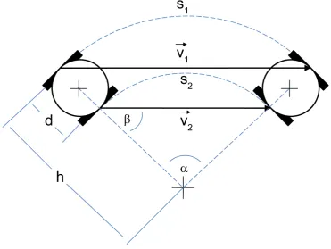
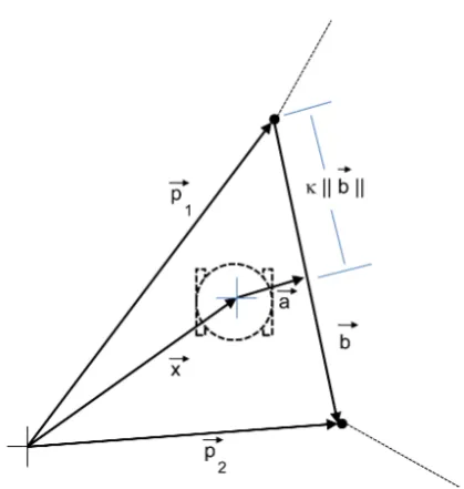
5.1 Diagram of variables for two-wheeled motion derivation . . . 46

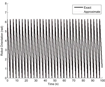
5.2 Verification of rotational accuracy with and without approximation. . . 49

(10)

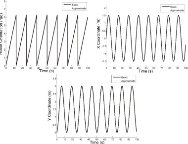
5.4 Verification of rotational and translational accuracy used the respective left and right wheel speeds of ν1 = 0.5 m/s and ν2 = 1 m/s. The maximum orientation,x-position, andy-position errors are 0.037 rad, 0.055 m, and 0.056

m, respectively. . . 51

5.5 Diagram of variables for obstacle collision check. . . 52

5.6 Collision detection was verified by placing the robot within a small obstacle and having it move around. As shown above, the center of the robot is never closer than 0.5 m (the radius) to the obstacle wall. . . 54

5.7 Model of robot sensor configuration for path following simulations. . . 54

5.8 Diagram of variables used for path detection calculations. . . 54

5.9 Model of robot sensor configuration for full 2-D navigation. . . 56

5.10 Diagram of variables used for full 2-D navigation. . . 56

5.11 Graphical verification of accurate laser/object interaction. A blue line indi-cates the corresponding ANN input is inactivate while red line indiindi-cates the corresponding ANN input has been activated. The concentric circles are in-dicative of the desired goal . . . 57

6.1 Preference function for position error in line following evaluation . . . 59

6.2 Robot path compared with desired path . . . 60

6.3 ANN controller for a line following robot . . . 60

6.4 Code used to make line following controller . . . 61

6.5 Goal sensor configuration for the obstacle avoiding robots. Detection is sepa-rated into left, center, and right. . . 62

6.6 Environment for tier 4 evaluation . . . 63

6.7 Environment for tier 5 evaluation . . . 63

6.8 ANN controller for obstacle avoidance . . . 64

6.9 Obstacle avoidance robot in a densely obstructed environment . . . 65

6.10 Obstacle avoidance robot in a environment with concave obstacle . . . 65

6.11 Code used to make obstacle avoidance controller . . . 66

(11)

6.13 Goal sensor configuration for swarming robots where a member of the swarm

can detect the goal. . . 67

6.14 A single swarming robot in an environment with a convex obstacle . . . 67

6.15 A single swarming robot in an environment with a star obstacle . . . 67

6.16 Two swarming robots in an environment with a star obstacle . . . 68

6.17 Two swarming robots in a large environment with various obstacles . . . 68

6.18 ANN controller for each swarming robot . . . 69

6.19 Steps showing the movement of an evolved swarm . . . 71

6.20 A single swarming robot in an environment with concave obstacle . . . 72

(12)

List of Tables

2.1 Universal tiers for adjusting fitness exponent (x) . . . 20

3.1 Desired output pattern for XOR logic-gate . . . 25

3.2 Tiers for adjusting fitness exponent (x) in robust XOR evolution . . . 25

3.3 Tiers for adjusting fitness exponent (x) in scalable parity evolution . . . 29

4.1 The statistical results for varying mutation rates while only using point mutations 35 4.2 Mutation rates for 3-dimensional sensitivity analysis with variables in bold are indicative of the chosen points on Figure 4.4 . . . 38

4.3 The statistical results for varying mutation rates across the mutation rate landscape given in Figure 4.4 . . . 38

4.4 Actions in executed genes . . . 41

6.1 Tier for adjusting fitness exponent (x) in line following evaluation . . . 59

6.2 Dominant logic for line following robots . . . 60

6.3 Tiers for adjusting fitness exponent (x) in obstacle avoidance evaluation . . 62

6.4 Logic test goal finding robots are required to pass before simulation. For this test, all LIDAR inputs are inactive . . . 63

(13)

Chapter 1

Introduction

1.1

Motivation

Artificial neural networks (ANNs) are able to solve mathematically ill-defined problems

with a network of computationally simple elements. Inspired by the architecture of the hu-man brain, McCulloch and Pitts (1943) modeled biological neurons as simple mathematical

units capable of comprising large networks. Turing (1950) described the plausibility of a complex computing machine being constructed from simple computational units. Hornik

et al. (1989) proved that with the proper architecture, an ANN composed of McCulloch-Pitts neurons can approximate any regular function within a finite space to an arbitrary

degree of accuracy.

The potential of ANNs has inspired their application in a wide range of fields. The

primary use of neural networks has been for classification purposes. Wu et al. (1993) and Odewahn et al. (1992) showed how ANNs can be used to classify malignant tumors in

mammograms and star types in telescopic images, respectively. Waibel (1989) found use of temporal ANNs in the realm of speech recognition. Atiya (2001) detailed how neural

networks can be capable tools for analyzing credit risk.

Neural networks have also been used for robotic control. Naito et al. (1997) argued the

nonlinearity and distributed information storage of ANNs make them attractive candidates for control. Biewald (1996) used a neural network controller for obstacle avoidance by

partitioning the problem into separate path planning and local navigation regions. Cui and Shin (1993) controlled multiple manipulators by using neural networks to approximate the

(14)

et al. (2001) used ANNs as controllers that are able to evolve alongside the morphology of the controlled robots. Yue and Rind (2006) used a neural network for object recognition in

an obstacle avoiding robot.

However, there are limits to what current ANN learning algorithms can accomplish.

Convergence of the widely used back propagation algorithm is dependent on network ar-chitecture and learning rates (Hecht-Nielsen 1992). The setting of these parameters require

significant expertise and a priori knowledge of the problem to be solved. Otherwise, the network is likely to converge to a non-optimal solution or be unduly influenced by the

se-quence of learning examples that are given (Sutton 1986). Furthermore, training session require large amounts of historical data and are computationally demanding.

Hebb (1949) posited a theory that biological neural networks adapt by repeated firing. As the activation of one neuron coincides with the activation of another several times,

the connection between the two strengthens in such a way that it becomes easier for the first neuron to excite the second. Perhaps the most well-known application of Hebbian

learning in an ANN is a Hopfield network. Hopfield (1982) proved that an ANN can use Hebbian learning to converge to a local minimum, thus making the network stable.

However, stability requires the network be symmetrical, with nodes being connected to each other with identical weights. Even if this constraint is not enforced, Hebbian learning

is a capable method for getting ANNs to classify data (Sanger 1989; Oja 1992; Dauc´e et al. 1998). However, these methods often converge to local minima and are not suited to finding

an global optimum.

Real-time reinforcement is yet another scheme for adapting network connections. Onat et al. (1998) showed how positive reinforcement can be used to strengthen connections

between neurons when the network is performing as desired. Chialvo and Bak (1999) showed how similar learning occur with negative reinforcement. Bosman et al. (2003) gave a more

generalized approach which combined Hebbian and reinforcement learning. However, as evident in the work of Sutton and Barto (1999), there are several learning parameters of

the reward function which must be tuned, and these values require expertise or trial and error to set correctly.

Because training ANNs is inherently a trial-and-error process, it was a natural extension to use a genetic algorithm (GA) to train them. Genetic algorithms, also known as

(15)

(1975), GAs are a machine learning paradigm in which the parameters of a possible design solution are varied over time to eventually find a viable solution. Furthermore, many

so-lutions are designed in parallel, and the parameters of one solution may be used, partly or completely, in the parameters of another. As a result, the design solutions within a GA

improve over time in a manner similar to biological evolution. Like ANNs, GAs have found applications in a wide range of fields such as circuit design in electrical engineering (Miller

et al. 1997), ligand bonding in chemistry (Morris et al. 1998), and granular composites in material science (Fraternali et al. 2009).

Most ANNs designed by evolutionary algorithms involved optimizing the weight of a set network architecture (Montana and Davis 1989; Eberhart and Kennedy 1995). Further

work focused on evolving the parameter of various different learning algorithms (Roy et al. 1999; Chen et al. 1999).

Eventually there was an emergence of GAs in which network architecture and connection weights are coevolved in a process known as neuro-evolution. Reed (1999) gives a good overview of many GAs which evolve network architectures through decomposition, where a large, fully connected network has connections and nodes removed. The shortcomings of

such schemes were addressed by Angeline et al. (1999) who offered GNARL as an alternative. According to Angeline, decomposition methods often become trapped at local network

minima, which causes them to suffer the same non-optimum finding deficiencies GAs were designed to overcome.

More current neuro-evolution efforts include NEAT by Stanley and Miikkulainen (2002), and AGE by Duerr et al. (2006). Both methods utilize genomes that represent the nodes and connections of ANNs. The genomes of NEAT explicitly contain the connection weights.

The three tiers of NEAT, gene tracking, speciation, and complexifying, have become so well studied and efficient that Stanley et al. (2005) managed to evolve networks in real time. In

AGE, the genome includes a section for each node that, when combined with the similar section of another node, determines the weight of connections. Both NEAT and AGE are

able to use evolution to construct networks capable of performing complex control tasks. However, the practical size of evolved networks is limited by the requirement that each node

of the network is directly represented in the genome.

There are applications where a large network is necessary, such as the Gammon project

(16)

backgammon player. Gammon looks at the current state of the board and possible moves for a given roll of the dice. It then uses the neural net to calculate which possible move for the

given dice roll would lead to the highest probability of winning, and moves accordingly. With 198 input units and 40 hidden neurons, it plays on a level even with the best backgammon

players in the world. If one were to design such a network with a genetic algorithm, the GA would have to be scalable.

One of the first examples of a scalable GA was introduced by Kitano (1990). In his sem-inal paper, he used matricies to represent ANN connection weights. He achieved scalability

by using single bits to represent small connectivity graphs and allowing recursion of such bits. As a result, a neural network could be represented more compactly with reasonable

modularity. Tufte and Haddow (2000) used a similar genome shorthand to evolve large digital circuits.

Theraulaz and Bonabeau (1995) have shown that the reuse of a small set of rules to create a phenotype is an effective alternative to storing and manipulating the large amount

of data that describes each individual directly. Bentley and Kumar (1999) have shown that indirect encodings produce solutions to design problems faster and better than their directly

encoded counterparts. Federici and Downing (2006) have shown that rule-based encoded designs are more robust as well. Grajdeanu (2007) evolved rules capable of making virtual

2-D organisms with interesting properties such as cell differentiation and repair. Yogev and Antonsson (2007) created 3-dimensional structures by evolving a set a rules which directs

how a single cell should grow through a process called embryogenesis.

Embryogenesis is best described as genetic programming (GP) applied to the evolution of instructions which in turn determines how an artificial embryo should grow (Garis 1992).

A genetic program is a genetic algorithm where the evolution is performed on a computer program. In its inception, Fogel et al. (1966) devised a way to use the evolutionary

pro-cess that allowed the recombination of a computer program into various configurations. Later, LISP programs were evolved by Koza (1989) to create programs which could discover

recursive expressions for numerical sequences and pattern recognition. O’Neill and Ryan (2001) went on to make grammatical evolution (GE), which was a scheme for how to do

genetic programming in any arbitrary language. However, in GP the program is the end result of evolution. It is when these programs are used to grow something else when true

(17)

Embryogenesis was applied to ANN evolution when Gruau (1992) created cellular en-coding (CE), which dictates how a network grows from a single cell. CE was able to create

a network of arbitrary size that is capable of detecting logical parity. However, as noted by Luke and Spector (1996), Gruau achieves much of his modularity by using a recursion rule

that results in generating nodes with identical inputs and outputs. While his networks are able to perform well for tasks requiring symmetry, his method performs poorly for networks

that require asymmetric weights.

Kitano (1995) used his compact representation to encode instructions for the growth

of virtual axions and dendrites in graphical ANN. His scheme also implemented cell differ-entiation. However, this application was geared more towards simulating the growth of a

biological neural network instead of creating ANNs for engineering purposes.

Astor and Adami (2000) expanded on the idea of growing neural networks by creating

NORGEV, a simulated wet chemistry set. Within their evolutionary algorithm, a network is grown from a single neuron by using cell chemistry and protein diffusion models. One key

distinction of their work is that the evolved proteins not only provide growth instructions for the network, but also halt growth. While this method is able to make large neural

networks, it can take excessive evolution time as much of the processing power is devoted to simulating chemical diffusion.

Since GAs have been applied successfully in control problems (Yakovenko et al. 2004; Vigraham et al. 2005; Dupuis and Parizeau 2008; Zhang et al. 2008) it may come as now

surprise that the synergy of GAs, ANN, and control is a current area of research. Naito et al. (1997) evolved ANN controllers for simulated Khepera (Harlan et al. 2001) robots. Lipson and Pollack (2000); Pollack et al. (2003) have had much success in evolving the morphology

and control of robots. Floreano et al. (2007) evolved a swarm of robots which learn complex communication behaviors. Yet, all of these methods use direct representations, and if one

were to evolve an ANN complex enough to control an autonomous vehicle(s) (Cremean et al. 2006; Murray 2007), one would need a large ANN and a scalable GA to create it.

While Calabretta et al. (1998) and Stanley et al. (2009) have implemented GA with some scalability, their designs scale by using predetermined modules and symmetries, which are

(18)

1.2

Outline

This thesis will detail the methodology, analysis, and implementation of a new genetic algorithm for neuro-evolution. Designs in the GA are grown via a set of variable-length rules that are decoded to create a C++ _{program. The C}++ _{programs used to create the ANNs}

have an If-CONDITION-Then-ACTION structure. Each program has multiple sections that cycle through all pairings of nodes with tests and actions of the form:

If Node α and/or Node β meet certain CONDITION(S), Then perform AC-TION(S).

The expected result is to create an encoding scheme that, like CE, can take advan-tage of modularity to create large networks. However, it will also use the innovations of

NORGEV to evolve a more controlled growth as well. Having the growth directed by C++ programs comprising various recombinations of If-Then statements instead of solutions of complex diffusion equations will lead to shorter evolution times. While Neuro-Evolution Using Recombinational Algorithms and Embryogenesis, or NEURAE, may seem akin to

the GE of Tsoulos et al. (2005), the work presented here is only superficially similar. Limit-ing the evolution to onlyIf-Then commands constrains the search while remaining flexible enough to explore highly productive regions of the solution space. Furthermore, the pro-grams generated by NEURAE are the rules for embryogenesis, which provide scalability

and produce modularity. Conversely, the programs created by conventional GAs are direct representations of an ANN, and do not exhibit such scalability or modularity.

This thesis will show that NEURAE is a unifying GA capable of accomplishing a wide range of neuro-evolutionary goals. Chapter 2 will introduce the methodology of NEURAE

after a brief background of artificial neural networks and genetic algorithms. Chapter 3 will show that NEURAE is capable of evolving two types of parity evaluators. The first is

a 2-input XOR gate with many network redundancies. The second is a parity gate of an arbitrary size. The first task has definitive exploration versus exploitation regions, which

simplifies the analysis of the evolved rules. Furthermore, it will be shown that modularity can be produced in a randomly changing environment, in opposition to Kashtan and Alon (2005). The second task can be directly compared to existing literature, particularly that

(19)

Chapter 4 will analyze how and why NEURAE works in an effort to make the evolution-ary process more efficient. Like evolutionevolution-ary algorithms themselves, many of the mutations

used in NEURAE where inspired by natural mutations. Experiments were conducted to verify if and how the artificial mutations actually enhance evolution as well as their

biologi-cal counterparts are theorized to do. Next is an analysis of the individual created in a good and failed evolution to see what differences lie on a genomic level. Finally, an investigation

was conducted to see how different conditions and actions are used, and how their removal affects the GA.

Chapter 5 will give the derivations of the formulas used to create the robotic simulations in Chapter 6. Chapter 6 will show how NEURAE is able to evolve robotic controllers in

deceptive design domains. NEURAE will easily make controllers for a line following robot, and obstacle avoiding robot, and a coordinated swarm without any changes to its core

(20)

Chapter 2

Methodology

2.1

Background

2.1.1 Neural Networks

An artificial neural network (ANN) is a computing paradigm which is a gestalt of simple

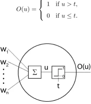
computational units called neurons or nodes. All ANNs in NEURAE are composed of McCulloch and Pitts (1943) modeled neurons. The input to each neuron is multiplied by

some scalar, or weight,wn. Next, the weighted inputs are summed and are in turn used as

the input,u, for a (usually) nonlinear activation functionO(·), as shown in Equation 2.1. In the original McCulloch-Pitts model, the nonlinearity could be any bounded function. Due to the desire to make learning algorithms easier to prove and implement, the activation

function usually forces the output of the neuron to be within [-1, 1]. This, however, is not a requirement and an activation function that bounds the output between 0 and 1 can be

used. Furthermore, digital networks usually use a discontinuous activation function while O(·) in an analog network would likely be continuous (Kartalopoulos 1996). Finally, neurons usually feature a constant, or bias, which is also summed to the inputs and serves to shift the activation function along the dependent axis.

u=

n

X

i=1

wi (2.1)

(21)

weighted before it is used as an input to another node,O(u) for an output neuron is always unweighted, resulting in a binary output for the entire ANN. The model of neurons used

in NEURAE is shown in Figure 2.1.

O(u) =  



1 ifu > t, 0 ifu≤t.

(2.2)

1 0

Figure 2.1: McCulloch-Pitts neuron model.

2.1.2 Genetic Algorithms

Genetic Algorithms (GAs) are a class of evolutionary computation, and repeatedly reiterate randomly created designs to find a desired solution. The design solutions are commonly

referred to as individuals, and the goal is to eventually create individuals that are capable of solving the design problem. Figure 2.2 is a simplified flowchart of the various steps contained

within a standard GA. GAs begin with an initial population of individuals with randomly created genomes. For all GAs there is a difference between the genotype and phenotype.

The genotype dictates the design parameters of the individual, and it is the altering of the genotype that ultimately alters the design parameters of the solution. The phenotype,

however, is the realization of the individual, and it is the phenotype which is evaluated. Thus, the individuals’ fitnesses are based upon how well their phenotypes complete the

design challenge.

However, the randomly created initial population is made up of poorly performing

(22)

eval-uation, selection, and mutation is repeated until either a prescribed time limit has passed or a good design is found.

Population Embryogenesis*

Evaluation

Selection Mutation

End

Figure 2.2: Steps of a standard genetic algorithm. (*Denotes an optional step).

The way individuals are represented, or encoded, within a GA is of paramount impor-tance to how they are evolved. As the encoding becomes more complex, the genotype to

phenotype mapping becomes a more involved process known as embryogenesis in which the phenotype starts as a small embryo, then grows according to its genome before or even during evaluation. Stanley and Miikkulainen (2003) offer classifications for the different

types of genomic encoding within present-day GAs.

• Direct -The design parameters of the phenotype are representeddirectly within the genotype. The approach works well for optimizing a design parameter, but the

one-to-one, genotype to phenotype relationship makes scalability a significant problem. Also, the lack of inherent modularity and symmetry makes it a poor candidate for

design synthesis.

• Developmental - The genotype is a compacted representation of the phenotype, and makes the phenotype by using a prescribed set of rules. This can scale well and

takes advantage of known modularity and symmetry. However, evolution is unable to discover and exploit unknown symmetries. Furthermore, the way modularity and

symmetry are used to compact genomic representation can unduly bias or even limit the solutions acquired.

(23)

an embryo. This approach offers the widest range of possible answers, and thus is the best method for generating completely novel designs. However, optimization is

ham-pered by the strongly non-injective mapping between the genotype and phenotype. Evolution times can also be slowed by extended periods of embryogenesis.

For NEURAE, an implicit encoding scheme was decided to place as little restriction as possible on the type of ANNs created. Thus, many of the examples of NEURAE exemplify

the creation of novel network architectures rather than the optimization of well-known ANN problems.

2.2

The NEURAE Genotype

2.2.1 Overview

Each individual in NEURAE is a digital, feed-forward neural network. However, the implicit encoding scheme of NEURAE means each ANN is created by the execution of the rules

encoded in its genome. When the genomes are decoded, the result is a C++ program. When the program is compiled and executed, the ANN is created.

The neural networks begin as a few neurons, but are grown according to the instructions encoded within their genomes. All ANNs start as the desired number of input neurons with

a threshold of 0. Each input node is able to create up to seven addition neurons. These subsequent neurons can exist within either the hidden or output layers, and can each make

up to seven addition hidden or output neurons. However, once the desired number of output nodes are created, the entire ANN is unable to create any additional neurons.

Each neuron can also make connections, and can continue to do so even after no more neurons can be created. To ensure the ANNs are feed-forward, nodes are only able to make

connections to neurons created after themselves. Furthermore, connections to any input node are prohibited. While nodes within the same hidden layer are unable to connect to

each other in most ANN applications, no such constraint is imposed here. Neurons within the hidden layer are able to connect to any other node within the hidden layer so long as

(24)

2.2.2 Biological Analog

A biological analogy was the inspiration for the encoding scheme used here. The genome of each individual is a variable-length array of integers which is decoded to create a C++

program. Every digit is analogous to a nucleotide whose value is inclusively between 1 and 100. A collection of six nucleotides forms a completeIf-CONDITION-Then-ACTION statement, and are analogous to a codon. These tests in the If-Then statements are not independent, and the sequence of codons will greatly influence how the individual will grow.

In particular, theIf-Thenstructure can be arranged such that multiple conditions are tested before an action can be executed. The closure of all If-Then statements, condition tests, and actions form a block analogous to a gene. The resulting (closed) If-Then statements in the C++ programs are similar toproteins. These concepts are shown in Figure 2.3.

.Nucleotide

1−1−15−15−10−26

| {z }

Codon

−40−38−2−1−95−16−100−1−2−3−4−5

| {z }

Gene

Figure 2.3: Sample genome and biological analog

2.2.3 If Structure Nucleotide

If Structure Test Value Action Type nucleotide nucleotide nucleotide

& ↓ .

1 - 1 - 15 - 15 - 10 - 26

% ↑

-Attribute Test Range Action Value nucleotide nucleotide nucleotide

w w

if(|Nodeα.ID1−B| ≤1 ) make.connection(-0.5)

Figure 2.4: Nucleotides of each codon

(25)

If-CONDITION-Then-ACTION tests can have a large effect on the computational process. This flexibility allows the GA to build complex algorithms from simple building blocks.

The logic corresponding to the numerical value of the first nucleotide is listed below.

• If -Opens anIf-Thenstatement. Adds action to the action stack. Nucleotides[1−25] • End-If - Writes in and removes last action placed into the action stack. Closes an If-Then statement. Opens another If-Then statement. Adds action to the action stack. Nucleotides [26−40]

• End-End-If - Writes in and removes last action placed into the action stack. Closes an If-Then statement. Executes and removes last action placed into the action stack stack. Closes anotherIf-Then statement. Opens an If-Then statement. Adds action to the action stack. Nucleotides [41−55]

• End -Writes in and removes last action placed into the action stack. Closes anIf-Then statement. Nucleotides [56−75]

• End-End - Writes in and removes last action placed into the action stack. Closes an If-Then statement. Executes and removes new last action placed into the action stack stack. Closes anIf-Then statement. Nucleotides [76−90]

• End-All - Writes in and removes last action placed into the action stack. Closes an If-Then statement. Repeats until all If-Then statements are closed. Nucleotides [91−100]

if(Testa)(Action A)

end-if(Testb)(Action B) end-iiff((TestTestb)a)((ActActiion on B)A) iiff((TestTestb)a)((ActActiion on A)B)

a a

A A

a

A B

B

b b b

B

B A if(a)

A end if(b)

B end

if(b) B end if(a)

A end

if(a) if(b)

B end A end

(26)

2.2.4 Condition Nucleotides

The next three nucleotides determine which of the ANN states that can cause actions to occur will be tested. The second nucleotide in each codon dictates which attribute will be

tested. The attributes are current states of Nodeαand/or Nodeβ. Many of these attributes affect the functionality of the neural network, such as the threshold of the neuron or the

number of connections it has. However, each node also has a three-part identification number that aids in evolution without affecting the functionality of the neuron. The first

part of the identification number (ID1) is denoted by a letter between A and H. Input nodes all have an ID1 of A and output nodes all have an ID1 of H. Hidden nodes can have an

ID1 of B through G, which is determined explicitly by the action which creates it. A node’s second ID number (ID2) is determined by the parent node which created it. If this is the

first node the parent node has made, the new node will have an ID2 of 1. If it is the third node the parent node has made, the new node will have an ID2 of 3. ID2 values can range

between 1 and 8 since any node can make, at most, 8 other nodes. ID3 values denote how many nodes within the entire network have the same ID1 and ID2 values. Thus the first node with an ID1 value of B and an ID2 value of 5 will have an ID3 value of 1, while the second node with the same ID1 and ID2 values will have an ID3 value of 2. These values

can range from 1 to 100. The result of the three different ID types is that each node will have a unique identification number.

The following list presents all possible node states which can be used by the attribute nucleotide. In addition to using the explicit values of Node α and/or Node β, relative differences between the two nodes can be considered as well. For values where a state of Node α relative to Node β orRel αβ are considered, the attribute of Nodeβ is subtracted from the value of the same attribute of Nodeα.

Similarly, there are options to consider the attributes of Node β relative to Node α, or Relβα. This can apply to all of the attributes listed above except for the connection weight. The value used for connection weight is the value of the weight from Node α to β or vice versa. The nucleotide ranges are for [Node α] [Node β] [Rel αβ] [Rel βα]. Equation 2.3 is used to get discrete values between ±1, excluding 0, wherezis the nucleotide and v is the value written into the C++ _program.

(27)

listed below.

• ID1 - Takes the ID1 value of a node, which can be between A and H. Nucleotides [1−5][27−31][53−55][77−79]

• ID2 - Takes the ID2 value of a node, which can be between 1 and 8. Nucleotides [6−10][32−36][56−58][80−82]

• ID3 - Takes the ID3 value of a node, which can be between 1 and 100. Nucleotides [11−14][37−40][59−61][83−85]

• Threshold - Takes the threshold of a neuron. Due to Equation 2.3, this can be a number in the range [-1−1]/0 in 0.02 increments. Nucleotides [15−17][41−43][62− 64][86−88]

• Number of Nodes Made - The number of subsequent nodes a node has made. Can be between 1 and 8. Nucleotides[18−20][44−46][65−67][89−91]

• Number of inputs - Number of inputs into a node. Can be between 0 and 99. Nu-cleotides[21−23][47−49][68−70][92−94]

• Number of outputs - Number of outputs from a node. Can be between 0 and 99. Nucleotides [24−26][50−52][71−73][95−97]

• Connection weight - Takes the weight of a connection between two nodes. Due to Equation 2.3, this can be a number in the range [-1−1]/0 in 0.02 increments. Nu-cleotides[74−76][98−100]

v(z) =   

 

z−50

50 if z≥51,

z−51

50 if z <51.

(2.3)

The third nucleotide writes the appropriate value into the test. In order for a condition test to return textit/true, the attribute (second) nucleotide must be within a certain range

of this test value nucleotide. The values written into the program depend on the attribute being tested. If the possible range is [0, 99], the number written into the program is the test value nucleotide minus 1. However, attributes that have only 8 possible values require

(28)

For threshold and connection values, Equation 2.3 is used if the attribute is a connection or the threshold of a neuron. However, if the attribute is the relative threshold of a neuron,

Equation 2.5, which gives a range of [0, 1.98], is used instead.

v=

z−1 12.5

, (2.4)

v(z) = z−1

50 . (2.5)

The fourth nucleotide determines the range over which the attribute can vary from the

test value and still have the condition return true. Similar to the test value nucleotide, the test range the nucleotide writes into the code depends on the attribute being tested. For

cases where letters are compared, this is the lexicographical range between the letters where two sequential letters have a lexicographical difference of 1.

2.2.5 Action Nucleotides

The final two nucleotides determine which actions are performed if the condition test is true. The fifth nucleotide determines which type of action will be placed into the action stack.

As mentioned above, the last in the “stack” of actions is written into the program whenever an If-Then statement is closed. Some nucleotides will result in the creation of a new node. Others will create a connection between Node α and Node β. In both these cases, the action value nucleotide dictates the threshold of the new node or weight of the connection,

respectively. The nucleotide-to-program transcription options are given by Equation 2.3. However, there are also No Action and End Turn action type nucleotides which will not insert any new action commands and end the pairing permutation, respectively. In these cases, the action value nucleotide is not used for anything. Figure 2.6 shows the genetic

string used to create a C++ program.

2.2.6 C++ _{Programs (Proteins)}

Each C++ program is a collection of proteins that build the phenotype. While the genome creates the bulk of the algorithm, there are a few rules hard-coded into the C++ program of every individual. These hard-coded rules are implemented to impose the minimum

(29)

Looping for pairing permutations

1-1-15-15-10-26

40-38-2-1-95-16

100-1-2-3-4-5 End ofgenome

{

Figure 2.6: Sample genome and protein pseudocode

a variety of architectures. First, the test statements described in the previous section are

always placed within twofor loops which cycle through all the different pairs of the ANN. Also, all of the inputs nodes have a ID2 value of 1. As there is no option to create another

input, each ANN will have the same number of input nodes.

However, there are also other mandatory conditions that must be met before an action

is executed, even if the CONDITION within the genome is true. For actions that make a connection, the first test is to make sure the two nodes are not already connected. Next, the process ensures that the neuron being connected to is not an input to the entire ANN, and

that the neuron being connected from is not the output for the entire ANN. Finally, there is a check that the neuron being connected to was made before the neuron which spawned

the connection to ensure the ANN is feed-forward.

To keep ANN size reasonable, ANNs have a limited amount of energy available for

growth. The act of creating a node or connection consumes one of the predetermined energy units for the entire ANN. Once a pairing executes an action that uses an energy

unit, that pairing is over. The individual is considered to be completely developed once the individual uses all 200 energy units or the programs cycles through all pairing permutations

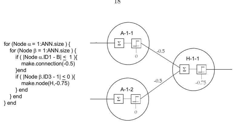
without performing any actions. Figure 2.7 shows the development of a NAND gate using the pseudo-code from Figure 2.6. It is important to note that an infinite number of different

(30)

A-1-1

A-1-2

H-1-1

Figure 2.7: Protein pseudocode and sample NAND gate

N N

N

N save =

α ∩ β α= 1

Start β= 1

a? b?

A? B?

A B

Y N

Y

β =

ANN end?

energy

--β= 1 energy

= 200

Y

N

β++

α =

ANN end?

save =

α ∩ β α∩β =

save?

energy > 0 ?

End

α= 1

α++

Y Y

Y N

N

LEGEND

a? = if ( |Nodeα. ID1 – B| < 1) b? = if ( |Nodeβ. ID3 – 1| < 0) A? = Is making a connection feasible? B? = Is making a node feasible?

A = Make a connection with weight of -0.5.

B = Make a node with ID 1 H and threshold of -0.75.

(31)

Step 1: Step 2:

EMBRYOGENESIS Neuron α= A-1-1 Neuron α = A-1-2

START Neuron β = A-1-1 Neuron β = A-1-1

Action: Make Node Action: None

0 A-1-1 0 A-1-2 0 A-1-1 0 A-1-2 0 A-1-1 0 A-1-2 -0.75 H-1-1

Step 3: Step 4: Step 5:

Neuron α = A-1-1 Neuron α= A-1-2 Neuron α = H-1-1 Neuron β = A-1-2 Neuron β = H-1-1 Neuron β = A-1-1 Action: None Action: Make Connection Action: None

0 A-1-1 0 A-1-2 -0.75 H-1-1 0 A-1-1 0 A-1-2 -0.75 H-1-1 0 A-1-1 0 A-1-2 -0.75 H-1-1 -0.5

Step 6: Step 7: Step 8:

Neuron α = H-1-1 Neuron α= H-1-1 Neuron α = A-1-1 Neuron β = A-1-2 Neuron β = H-1-1 Neuron β = A-1-1 Action: None Action: None Action: None

0 A-1-1 0 A-1-2 -0.75 H-1-1 -0.5 0 A-1-1 0 A-1-2 -0.75 H-1-1 -0.5 0 A-1-1 0 A-1-2 -0.75 H-1-1 -0.5

Step 9: Step 10:

Neuron α = A-1-1 Neuron α= A-1-1 EMBRYOGENESIS Neuron β = A-1-2 Neuron β = H-1-1 FINISHED

Action: None Action: Make Connection

0 A-1-1 0 A-1-2 -0.75 H-1-1 -0.5 0 A-1-1 0 A-1-2 -0.75 H-1-1 -0.5 0 A-1-1 0 A-1-2 -0.75 H-1-1 -0.5 -0.5

(32)

2.3

Evaluation, Mutation, and Selection

Each ANN is evaluated after the embryogenesis of each individual, as described by the method above. Evaluations in NEURAE are performed in tiers to ensure network feasibility and to promote evolution of complex behaviors (Graham et al. 2009).

The first tier ensures the individual grows the correct number of output nodes. If the correct number of outputs are made, the individual advances to the second tier, where the

exponent is increased for each output node with a connection. These two requirements, listed in Table 2.1, are the minimum for any possibly viable ANN circuit, and once met,

will yield an exponent value ofx−1 = 1. The remaining tiers vary depending on the design problem, and are listed alongside the design problem to which they pertain.

Table 2.1: Universal tiers for adjusting fitness exponent (x)

Tier Test Change in Exponent 1 Are there enough

output nodes?

fraction of desired output nodes

2 Are there a connec-tions to each out-put node?

+ fraction of output nodes with connec-tions

Another commonality all evaluations share is the fitness function shown in Equation 2.6. While x is a linear comparison of two individuals, the exponential nature of Equation 2.6 magnifies any improvements and greatly improves convergence in NEURAE. Furthermore, the floor function ensures individuals which are unable to pass the first tier have zero fitness,

virtually nullifying their odds of survival.

Fitness =2x−1. (2.6) A roulette style of selection determines which individuals are used for creating the next generation. The population size in each generation is conserved. The probability of selecting

an individual is determined using Equation 2.7; where Pi, fi, and N are the probability

(33)

mutation, conjugation, translocation, genome replication, and genome deletion.

Pi =

fi

PN

j=1fj

. (2.7)

As described by Holland (1992), classical GAs change the genotype of future populations

through point mutation and crossover of current individuals. Figure 2.10 shows an example of a point mutation in a binary genome where a random bit is flipped. Point mutations

are also used in NEURAE, but instead of a binary bit flip, a random nucleotide is replaced with a randomly chosen integer inclusively between 1 and 100.

111000111000 ⇒ 110000111010

Figure 2.10: Point mutation example. The underlined nucleotides are switched

Crossover mutations require two individuals to make two more individuals and are

usu-ally either single-point or two-point crossover. With single-point crossover, two individuals make two new individuals by having their genomes broken and swapped at a random

loca-tion on the genetic string. In two-point crossover, only a secloca-tion of the genomes are swapped. Figures 2.11 and 2.12 give an example of both types. For GAs in which all genomes must

be the same size, the sections to be swapped must be of identical length. Furthermore, the sections are usually at the same genome locus such that the information being exchanged

at that locus has some correlation to its purpose in the phenotype. In NEURAE, however, there is little correlation between the functions of the same section of genome between two

different individuals. Furthermore, while crossover may produce one improved individual, they seldom create two. Thus, genetic material is shared during mutations in NEURAE

through a process inspired by, and named after, biological conjugation.

111000111000

⇒ 111000101010 101010101010 101010111000

Figure 2.11: Single-point crossover mutation example. Parts of the genome which have been swapped are underlined

111000111000

⇒ 111010101000 101010101010 101000111010

Figure 2.12: Two-point crossover mutation example. Parts of the genome which have been swapped are underlined

In biology, conjugation is a process used by many species of bacteria where one bacterium

(34)

exchange may have been key in the evolutionary jump from prokaryotes to eukaryotes and Jain et al. (1999) and Ochman et al. (2000) offer conjugation as a reason for the high

adaptability of present-day bacteria. NEURAE uses conjugation in the manner shown in Figure 2.13, where a section of one genome is inserted into the genome into another. Thus,

new rules can be exchanged between individuals and, hopefully, the benefits of biological conjugation can also be used by NEURAE.

111000111000

⇒ 1110001010111000 10101010101010

Figure 2.13: Conjugation mutation example. Parts of the genome which have been inserted are underlined

Ohno (1970) introduced the concept of genome duplication as another key component of biological evolution. During replication, portions of the genome are at times copied more

than once, resulting in an offspring that has two genes which make the same protein. Ohno theorized this redundancy made the individual more robust to future mutations, because if

one gene became non-functional, there is another copy to do the same job. This redundancy was also noted by Britten (2005), who observed that many sections of the human genome have sequences that are too similar to have arisen independently. NEURAE uses a genome

duplication process as shown in Figure 2.14, where a section of a genome is copied more than once when it is being replicated.

111000111000 ⇒ 111000111111000

Figure 2.14: Gene duplication example. The nucleotides copied more than once are underlined

The final two mutation types are gene deletion and translocation. In gene deletion a section of the genome is removed during replication. While gene deletion is an observable

phenomenon in biology, its effects are usually damaging (Lewis 2005). However, it was added as a mutation here to counter the concatenating effects of conjugation and gene

duplication. Translocation, where a section of the genome is moved to another locus, is yet another observed biological mutation. Regardless of its implications to biological evolution,

(35)

show examples of these two processes in NEURAE.

111000111000 ⇒ 111000000

Figure 2.15: Gene deletion example. The nucleotides deleted are underlined

111000111000 ⇒ 111111000000

Figure 2.16: Translocation example. The underlined nucleotides are moved to another gene locus

Finally, it was necessary to prevent frame-shift mutations. A frame-shift mutation adds or deletes only part of a codon. The result is a shift in nucleotides that causes all following

(36)

Chapter 3

Logic-Gate Evolution

3.1

Overview

This chapter will describe how NEURAE creates logic gates. Each evolutionary run begins

with the random creation of 200 individuals for 1000 generations. These values were found to give good results in run times around 4 hours on a cluster of 25 dual quad-core, 2.33 GHz

computers. Furthermore, each individual started with a genome 300 nucleotides (50 codons) long. During evolution, a genome is allowed to double in size before being trimmed to the

default length. Genome length was constrained to prevent the well-documented problem of bloat in genetic programming (Koza 1992; Langdon 2000). While this arbitrary setting

of genome length may bias evolution, Szathm´ary and Smith (1995) have evidence showing that overall genome length of a biological organism has little to do with the complexity of

the phenotype.

The first goal is to evolve an ANN that can serve as an XOR logic gate (Table 3.1),

even if the ANN suffers multiple failures. This circuit was chosen because its nonlinearity requires the creation of a hidden layer and is a common benchmark in the evolution of ANN

logic circuits (Koehn 1996; Ashlock 2006). The next logic gate to be evolved is a parity gate. A parity gate is a standard logic circuit used in simple error detection. An even parity logic

(37)

Table 3.1: Desired output pattern for XOR logic-gate

Input 2 0 1

Input 1 0 0 1 1 1 0

3.2

Robust XOR Gate

3.2.1 Evaluation Parameters

Table 3.2 shows the tiers used in evaluating the evolved XOR gates, the exponent gets an

additional point for each correct answer. If an individual is able to get to the third tier, the exponent in Equation 2.6 has a value of x−1 = 1. At this point, the network’s truth table is compared with that of the desired circuit in tier 3. If the individual passes tier 3 and is a functional XOR gate, x = 6 and the individual will have an overall fitness of 32. In tier 4, a node is randomly removed, and the ANN is compared to the target XOR logic again. Nodes are continually removed until the circuit no longer produces the target logic.

This test for robustness is performed for each generation the individual is alive. Because the order in which the nodes are removed changes with each generation, the fitness of an

individual is not constant, and the overall robustness will increase.

Table 3.2: Tiers for adjusting fitness exponent (x) in robust XOR evolution

output nodes?

3 Compare to the de-sired truth table

+ # of correct an-swers in each table entry

4 Break nodes until failure

(38)

3.2.2 Evolution Results

Figure 3.1 shows the fitness of the best individual of each generation. Figure 3.2 shows the first XOR gate synthesized by evolution in generation 823, and Figure 3.3 shows how it

functions. In these figures, a node is filled-in (black) when it is activated. A solid connection indicates a positive weight while a dashed connection is indicative of a negative weight. As

shown in Figure 3.3, the activation of either input will activate only the output. Once both nodes are on, three of the four hidden nodes are activated, and their inhibitory connections

to the output are enough to deactivate it. However, this ANN is not robust, as all three hidden nodes are needed to counter the activation of both inputs, and the removal of any

one will break the entire ANN.

Generation

B

es

t F

itn

es

s

Figure 3.1: Best fitness throughout the evolution of a robust exclusive-OR logic gate

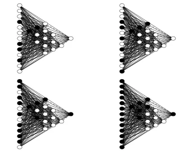
By the end of the evolutionary run, a much larger ANN was created and is shown in Figure 3.4. This ANN comprises 49 nodes and 140 connections. The algorithm created this

ANN by taking the smallest possible XOR gate (shown in Figure 3.5) and making duplicate copies of it. The resulting ANN can have all but one hidden node removed, and is as robust

to node removal as possible. Furthermore, the ANN used 189 out of the 200 possible energy units, making it close to the maximum size this evolution would allow.

Nevertheless, this is not the largest, fully redundant ANN this genetic algorithm could have made. Figure 3.6 shows a refined version of the individual’s code, which shows only

(39)

I

nput

Nodes

Hi

dden

Nodes

Out

put

Node

Figure 3.2: First generated XOR gate Figure 3.3: Network functionality

(40)

the output node, which in turn halts all further neuron growth. If the test value is increased from 3 to 5, and the maximum number of energy units available for growth is not limited,

then the 195 node network shown in Figure 3.7 is produced.

Figure 3.6: Code for creating a robust XOR

gate Figure 3.7: Larger XOR gate

The results of this experiment show that NEURAE is able to create large and complex

network structures. Not only is this GA able to solve the standard benchmark in logic neuroevolution, it was able to expand on it by finding the core module and replicating it.

The ability of NEURAE to construct large networks with such regular structure will be key for future applications.

3.3

Large Parity Gate

3.3.1 Evaluation Parameters

Table 3.3 shows that for the creation of a variable-size parity gate, the exponent is increased

(41)

Table 3.3: Tiers for adjusting fitness exponent (x) in scalable parity evolution

output nodes?

3 Compare to the de-sired truth table

+ fraction of correct answers in each table entry

3.3.2 Evolution Results

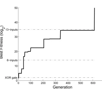
The genetic algorithm was also able to create a parity gate for an arbitrary number of

in-puts. Figure 3.8 shows the fitness of the best performing individual throughout evolution. The particular evolutionary run shown here produced a 2-input parity (i.e., XOR) gate

much more quickly than the run shown in the previous section. This large variability is a by-product of the stochastic nature of GAs. At the 621st generation, NEURAE finally

generated a fully scalable individual. However, the discovery of this individual resulted in

the halting of the GA due to the excessive time required to evaluate 21 X

n=2

2ninput

configura-tions. While a more elegant evaluation method could have circumvented this issue (Gruau

1994), the fact still remains that NEURAE was able to solve the problem at hand.

As shown in Figure 3.9, the 2-input parity gate works by having hidden nodes which

inhibit the output once both input nodes are activated. The hidden nodes, however, also inhibit the activation of other hidden nodes that were made afterwards. This cascading effect can also be seen in the 4-input parity gate shown in Figure 3.10. The internal cascading

structure of the 2-input network is able to scale accordingly to the 4-input network by having the number of hidden nodes equal the number of output nodes. Having two inputs active

in the 4-input gate is identical to having two inputs active in the 2-input gate. Activating a third input is able to turn on the output node without activating another hidden node.

However, the activation of a fourth input activates another hidden node, which in turn is sufficient to inhibit the excitation of all four inputs. Figure 3.11 shows this cascading effect

scales with the number of inputs in an ANN with 13 inputs.

(42)

Gener

at

i

on

B

es

t F

itn

es

s

(lo

g

)

₂

Figure 3.8: Fitness of best-performing individual throughout the evolution of a scalable parity gate

(43)

Figure 3.10: Scalable parity gate with four inputs 0 0.1 0.2 0.3 0.4 0.5 0.6 0.7 0.8 0.9 1 0 0.1 0.2 0.3 0.4 0.5 0.6 0.7 0.8 0.9 1 0 0.1 0.2 0.3 0.4 0.5 0.6 0.7 0.8 0.9 1 0 0.1 0.2 0.3 0.4 0.5 0.6 0.7 0.8 0.9 1 0 0.1 0.2 0.3 0.4 0.5 0.6 0.7 0.8 0.9 1 0 0.1 0.2 0.3 0.4 0.5 0.6 0.7 0.8 0.9 1 0 0.1 0.2 0.3 0.4 0.5 0.6 0.7 0.8 0.9 1 0 0.1 0.2 0.3 0.4 0.5 0.6 0.7 0.8 0.9 1

(44)

twice the magnitude of a positive connection. Thus the excitation of two input nodes is canceled out by the excitation of one hidden node. Furthermore, as the network begins

with more inputs, the number of hidden nodes made during embryogenesis increase as well, providing scalability.

Once again, certain hard limits prevent parity gates of any arbitrarily large size to be created. First, a limit of 200 energy units prevents this network from growing a parity gate

with more than 13 inputs. Also, the 99 connection limit placed on the maximum number of inputs and outputs caps the parity gate size at 66 inputs. Fortunately, both these limits

were established only to help the evolution process and can be increased as necessary to allow the code in Figure 3.12 to create parity logic for an arbitrary number of inputs.

(45)

Chapter 4

Sensitivity Analysis

4.1

Mutation Rates

Many of the values used for the genetic algorithm were heuristic. Fortunately, NEURAE is

able to solve the robust XOR problem with a wide range of values. Still, as the design chal-lenges for NEURAE become more difficult, it is important to not disadvantage NEURAE

by using suboptimal evolutionary parameters. Some parameters, such as population size and number of generations per evolution, are dependent on the computer resources

avail-able. However, the mutation rates were arbitrarily chosen, and are likely not the optimum. Furthermore, these mutation values can be adjusted independently of the hardware used

and, hopefully, independently of the problem being solved.

NEURAE has a two-step process in determining mutations. After an individual is

selected to produce offspring, its genome is scanned using the overall mutation rate, µ ∈ [0,1]. Each codon has a probability µ of undergoing some type of mutation. Based on this random selection, when a mutation will occur, NEURAE then randomly selects from the secondary mutation options the type of mutation the codon will undergo. The possible

mutations of point, conjugation, duplication (recopy), deletion, and translocation have the respective rates of µP, µC, µR, µD, and µT.

In order to determine the appropriate balance of the various mutation rates, a series of experiments were conducted. Each series was composed of ten evolutionary runs. Because

the creation of an XOR gate is feasible by using only point mutations, a series of tests were run to determine the optimal point mutation rate. These tests set the µP rate to

(46)

highest-scoring individual at the end of evolution.

Statistical data for the first generation in which an XOR gate was made, orαgeneration, was fitted to a two-parameter Weibull distribution (Weibull 1951). A Weibull distribution has the cumulative distribution function (CDF) and probability distribution function (PDF)

given in Equations 4.1 and 4.2, respectively. In these equations, k is the shape parameter and λ is the scale parameter. These parameters were found by performing a least-squares line-fit on the data shown in Figure 4.1, where the slope of the line isk, and the x-intercept is λ. Once these values are found the integral of the PDF (Equation 4.2) is used to determine the likelihood of an XOR gate will being created within 1000 generations.

F(x) = 1−e−(x/λ)k, (4.1)

P(x) = k λ

x λ

k−1

e−(x/λ)k. (4.2)

αgeneration

ln

1 _1-F

(

)

__

_

Figure 4.1: Log-log plot of α generation vs. log₁₋1_F for a point mutation rate of µ= 0.4.

αgeneration

P

D

F

Figure 4.2: Probability density function and histogram ofα generation for muta-tion rate ofµ= 0.4.

The Ω fitness is the fitness of the best performing individual at the end of the

evolu-tionary run. Because cases where an XOR is never found are capped at 16, those runs are excluded to focus on the exploitative effects of the mutation rates. This statistical data was

found to be best fit to a Gaussian distribution, as shown in Figure 4.3.

Table 4.1 illustrates that evolutions using mutation rates at the extremes are both less

(47)

75 80 85 90 95 100 105 110 115 120 125 0

0.5 1 1.5 2 2.5 3 3.5 4 4.5 5

Figure 4.3: Gaussian distribution of best fitness at the end of evolutionary runs with a point mutation rate of µ= 0.4.

Table 4.1: The statistical results for varying mutation rates while only using point mutations

Case µ Probabilityα gen≤ 1000 Ω fit mean Ω fit st. dev.

1 0.05 73.1% 99.67 10.36

2 0.1 90.2% 108.8 7.26

3 0.2 92.9% 106.0 8.40

4 0.4 97.3% 101.1 10.12

5 0.6 99.5% 97.39 23.64

6 0.8 99.1% 94.35 18.47

(48)

with other literature which shows that extremely high and low mutation rates are often deleterious to GAs (M¨uhlenbein 1992; B¨ack and Schutz 1996).

However, mutation rates between 0.1 and 0.8 offer a trade-off between the likelihood of finding an XOR gate and optimizing an ANN. As shown in Table 4.1, a higher mutation

rate makes finding an XOR gate more likely. However, lower mutation rates are generally more capable of exploiting a functional XOR design and making it robust. Thus, a user

can either decide whether the problem being solved is more explorative or exploitative in nature, and chooseµP accordingly, or use variable mutation rates, such as those shown by

McGinley et al. (2008).

It may be possible to improve both the explorative and exploitative capabilities of

NEU-RAE without using a variable mutation rate which comes with its own biases and problems (B¨ack 1992). It was hoped that other mutations found in nature would be beneficial to

include in NEURAE as well. As mentioned in Chapter 2, NEURAE is capable of altering newly created genomes using mutations besides simple point mutations. A sensitivity

anal-ysis was conducted to determine the appropriate rates of the rest of the mutation types. However, the mutation rates are interdependent, so the sensitivity analysis was

adminis-tered in a manner detailed by Montgomery (2004) for studying the effects of dependent variables. Overall, there are 6 variables. However, there are a few constraints that reduce

the degrees of freedom.

The first constraint, Equation 4.3, requires the probability of a point mutation to be

held at 0.4. The value of 0.4 was chosen because it is in the middle of the plateau of mutation rates that perform well. Furthermore, the previous experiments prove that the overall mutation rate can be increased without adversely affecting NEURAE.

µ·µP = 0.4. (4.3)

Next, the secondary mutation rates must sum to 1, as shown in Equation 4.4. This is to ensure that a mutation happens as the overall mutation rate,µ, dictates. The constraint shown in Equation 4.5 was added because the operations of crossover and gene duplication

lengthens the genome while deletion shortens it. Having the mutation rates of these oper-ations balanced makes sure the genomes’ lengths are not unduly biased. This constraint,

(49)

µ

C

µ

R

0 0

1.0

0.6

8

14

13

12

11

10

9

1 -µ_P

2

1 -µ_P

2

Figure 4.4: The prism is representative of the mutation rate landscape as bounded by the above constraints.

inequality in Equation 4.6.

µP +µC +µR+µD+µT = 1.0, (4.4)

µC+µR=µD, (4.5)

µC+µR≤

1−µP

2 . (4.6)

These constraints can be used to create the mutation rate landscape shown in Figure

4.4 and a 3-dimensional sensitivity analysis can be performed by varying µ, µC, and µR

with data taken at the corners and centroid of the prism to maximize the exploration of the

mutation rate landscape. Table 4.2 shows the values used for exploring the mutation rate landscape, which are at the corners and centroid of the prism shown in Figure 4.4.

Table 4.3 offers the results of the mutation rate sensitivity analysis. In general, the excessively high mutation rates (µ = 1.0) were once again the poorest performing.

Fur-thermore, cases that use only point mutations and genome size changing mutations (i.e., conjugation, duplication, and deletion) perform worse than using point mutations alone.

(50)

Table 4.2: Mutation rates for 3-dimensional sensitivity analysis with variables inbold are indicative of the chosen points on Figure 4.4

Case µ µP µC µR µD µT

8 0.6 0.66 0.0 0.0 0.0 0.34 9 1.0 0.40 0.0 0.0 0.0 0.60 10 0.6 0.66 0.17 0.0 0.17 0.0 11 1.0 0.40 0.30 0.0 0.30 0.0 12 0.6 0.66 0.0 0.17 0.17 0.0 13 1.0 0.40 0.0 0.30 0.30 0.0 14 0.8 0.5 0.075 0.075 0.15 0.20

rate, as was done in case 8, achieved good results. Still, there is a delicate balance between these values since case 9, which also only used point and translocation mutations, was by

far the worst performing test case. This case only had two of the 10 runs produce an XOR gate. Nevertheless, the best combination of mutations rates is case 14, which uses all of the

mutation types. These runs have a high probability of discovering an XOR gate (99.95%) coupled with good optimization. As a result, this became the balance of mutation rates

used for future design problems.

Table 4.3: The statistical results for varying mutation rates across the mutation rate land-scape given in Figure 4.4

Case Probability α gen≤1000 Ω fit mean Ω fit St. Dev.

8 97.3% 106.6 8.48

9 19.1% 75.7 40.6

10 86.1% 92.99 18.84

11 56.6% 100.8 8.95

12 71.8% 98.34 10.52

13 56.5% 92.95 5.48

14 99.95% 102.8 10.60

4.2

Qualities of Productive Evolution

(51)

using only point mutations, but one case had a moderate mutation rate (µ= 0.2, µP = 1.0)

which often produced XOR gates. The second group had a higher mutation rate (µ =

0.8, µP = 1.0) which seldom produced an XOR gate. Characteristics of successful, XOR

producing runs were compared to those of non-XOR producing, unsuccessful runs. While

the quantitative results differ between the two groups, the qualitative results for each group are similar.

B

es

t F

itn

es

s

G

en

e

N

um

be

r

Generation

Figure 4.5: Genes used by the top 10% within a successful evolution

Generation

B

es

t F

itn

es

s

G

en

e

N

um

be

r

Figure 4.6: Genes used by the top 10% within an unsuccessful evolution

Figures 4.5 and 4.6 show which genes were used by the best individuals (top 10%) throughout evolution. Each time a gene is used, a dot is placed that shows in which

generation it was used. Furthermore, the figure is overlaid with a plot of the fitness of the best performing individual of each generation.

In Figure