Endoscopic Optical Coherence Tomography: Design and Application

(1)

Endoscopic Optical Coherence Tomography:

Design and Application

Thesis by

Jian Ren

In Partial Fulfillment of the Requirements for the Degree of

Doctor of Philosophy

California Institute of Technology Pasadena, California

2013

(2)

(3)

(4)

Acknowledgments

This dissertation would not have been made possible without the help, support, and encouragement from a group of amazing people who enabled me to make this labor of intellectual curiosity possible. I am fortunate to have had such a tremendous experience, both as a researcher and a professional. I am grateful to all who have helped me along the way.

My greatest appreciation goes to my advisor, Professor Changhuei Yang. I am thankful to him for introducing me to the interesting area of biomedical optical imaging. His expertise allowed me to rapidly immerse myself in this area; his vision and insight constantly inspired me in my research. More importantly, his intensive enthusiasm to the pursuit of engineering and science has always been motivating me to think creatively and act courageously.

Many other faculty members also had an impact on my work. I am indebted to Professor Mark Humayun, who was invaluable during the early stage of my research in ophthalmic imaging. He, too, frequently pointed me towards new opportunities. I would also like to thank Professor Yu-Chong Tai, Professor Azita Emami, Professor Chin-Lin Guo and Professor Hyuck Choo for being my committee and giving me many valuable suggestions.

To Jeff Brennan, who provided me both funding and access to the resources that are imperative for my research in the last two years, I give my sincere thanks. I have been greatly energized by his unmatched enthusiasm for both my dissertation and our collaboration. I am grateful for the opportunity of offering me a platform for interdisciplinary research.

And I would like to pay my heartiest thanks to my colleagues and friends at Caltech for their friendship and for the numerous technical discussions that inspired and continue to inspire my work throughout my graduate study. A far from complete list includes Qiang Lin, Jigang Wu, Xiquan Cui, Emily McDowell, Guoan Zheng, Shuo Pang, Ying Min Wang, Chao Han, Mooseok Jang. Ya-Yun Liu, Christine Garske, Agnes Tong, and Anne Sullivan have been helping me with many purchasing and administrative matters.

(5)

Abstract

This thesis presents an investigation on endoscopic optical coherence tomography (OCT). As a noninvasive imaging modality, OCT emerges as an increasingly important diagnostic tool for many clinical applications. Despite of many of its merits, such as high resolution and depth resolvability, a major limitation is the relatively shallow penetration depth in tissue (about 2∼3 mm). This is mainly due to tissue scattering and absorption. To overcome this limitation, people have been developing many different endoscopic OCT systems. By utilizing a minimally invasive endoscope, the OCT probing beam can be brought to the close vicinity of the tissue of interest and bypass the scattering of intervening tissues so that it can collect the reflected light signal from desired depth and provide a clear image representing the physiological structure of the region, which can not be disclosed by traditional OCT. In this thesis, three endoscope designs have been studied. While they rely on vastly different principles, they all converge to solve this long-standing problem.

A held endoscope with manual scanning is first explored. When a user is holding a hand-held endoscope to examine samples, the movement of the device provides a natural scanning. We proposed and implemented an optical tracking system to estimate and record the trajectory of the device. By registering the OCT axial scan with the spatial information obtained from the tracking system, one can use this system to simply ‘paint’ a desired volume and get any arbitrary scanning pattern by manually waving the endoscope over the region of interest. The accuracy of the tracking system was measured to be about 10 microns, which is comparable to the lateral resolution of most OCT system. Targeted phantom sample and biological samples were manually scanned and the reconstructed images verified the method.

Next, we investigated a mechanical way to steer the beam in an OCT endoscope, which is termed as Paired-angle-rotation scanning (PARS). This concept was proposed by my colleague and we further developed this technology by enhancing the longevity of the device, reducing the diameter of the probe, and shrinking down the form factor of the hand-piece. Several families of probes have been designed and fabricated with various optical performances. They have been applied to different applications, including the collector channel examination for glaucoma stent implantation, and vitreous remnant detection during live animal vitrectomy.

(6)

EO effect of a KTN crystal. With Ohmic contact of the electrodes, the KTN crystal can exhibit a special mode of EO effect, termed as space-charge-controlled electro-optic effect, where the carrier electron will be injected into the material via the Ohmic contact. By applying a high voltage across the material, a linear phase profile can be built under this mode, which in turn deflects the light beam passing through. We constructed a relay telescope to adapt the KTN deflector into a bench top OCT scanning system. One of major technical challenges for this system is the strong chromatic dispersion of KTN crystal within the wavelength band of OCT system. We investigated its impact on the acquired OCT images and proposed a new approach to estimate and compensate the actual dispersion. Comparing with traditional methods, the new method is more computational efficient and accurate. Some biological samples were scanned by this KTN based system. The acquired images justified the feasibility of the usage of this system into a endoscopy setting.

(7)

List of Figures

1.1 Simplified OCT system setup using a fiber based Michelson interferometer. . . 5

2.1 Illustration of mechanical and manual scanning . . . 23

2.2 Image artifact induced by non-uniformity of hand motion. . . 23

2.3 Schematic of the tracking system. . . 24

2.4 Workflow of the OCT tracking system . . . 25

2.5 Schematics of the hand-held probe . . . 25

2.6 Tracking accuracy characterization . . . 26

2.7 Target phantom OCT image . . . 28

2.8 Tadpole OCT image by manual scanning . . . 29

2.9 3D scan patterns . . . 29

3.1 The principle of PARS scanning . . . 33

3.2 Implementation of PARS probe . . . 33

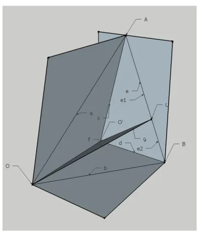
3.3 PARS scan geometric configuration . . . 34

3.4 Comparison between the new and the old model . . . 36

3.5 Comparison between ZEMAX simulation and the new model for deflection angle . . . 37

3.6 Simulated off-plane angle . . . 37

3.7 Scan pattern comparison. . . 38

3.8 Experimental measurement of deflection angle dependency . . . 38

3.9 21/23 gauge hand-held probe . . . 39

3.10 Tubing Assembly for 21/23 gauge hand-held probe . . . 40

3.11 Schematics of the outer needle . . . 40

3.12 Schematics of the inner needle . . . 41

3.13 Schematics of the rotary jointer . . . 41

3.14 System function diagram . . . 42

3.15 Photography of prototype hand-held PARS probe . . . 43

4.1 Glaucoma stent implantation and imaging guidance by an endoscopic OCT probe. . . 46

(10)

4.3 A side view of the endoscopic OCT probe and actuation system . . . 48

4.4 The swept source OCT setup. . . 49

4.5 OCT and SEM images of human cadaver eye tissue segments. . . 51

4.6 The relationship between deflection angleθand rotation angle ξ. . . 53

4.7 Illustration of the vitrectomy procedure . . . 54

4.8 Illustration of PARS aiding vitrectomy . . . 55

4.9 PARS probe imaging an enucleated porcine eye . . . 55

4.10 OCT image of optical nerve and blood vessel . . . 56

4.11 Comparison of vitreous and saline. . . 56

4.12 Sub-retinal bubble . . . 57

4.13 Vitrectomy on live rabbit . . . 58

4.14 OCT images of vitrectomized rabbit . . . 58

5.1 KTN Principle . . . 63

5.2 Space-charge-controlled EO effect principle diagram . . . 64

5.3 Structure of the KTN deflector . . . 65

5.4 Structure of the KTN scanner . . . 65

5.5 Deflection angle versus applied voltage . . . 66

5.6 KTN crystal current consumption . . . 66

5.7 The relay telescope for bench top KTN OCT setupn . . . 67

5.8 Photograph of the bench top relay telescope . . . 67

5.9 Swept source OCT setup used in the KTN experiment . . . 68

5.10 Profile of the bench top KTN OCT probing beam . . . 69

5.11 Point spread functions of the KTN OCT system . . . 70

5.12 Beam quality of the KTN OCT system . . . 71

5.13 Gaussian beam parameters . . . 71

5.14 Beam focus displacements of the KTN OCT system. . . 72

5.15 Beam focus trajectory of the KTN OCT system . . . 73

5.16 Human finger skin OCT image by KTN scanning . . . 74

5.17 OCT image of a ex-vivo porcine eye retina . . . 74

5.18 OCT images of a 54 stage Xenopus laevis tadpole by the bench top KTN system . . . 75

5.19 Schematics of endoscopic probe based on KTN deflector . . . 76

6.1 Instability of metric function based methods . . . 82

(11)

List of Tables

3.1 Form factor comparison . . . 42

5.1 KTN 2-D module operating temperature . . . 65

5.2 Reflected power measurement . . . 68

(12)

Nomenclature

CT computed tomography

PET positron emission tomography

OCT optical coherence tomography

NA numerical aperture

GRIN gradient indexed

MRI magnetic resonance imaging

KTN potassium tantalate niobate

PSF point spread function

NDT non-destructive test

FWHM full width half maxim

PNS peripheral nerve stimulation

(13)

Chapter 1

Introduction

Dependable diagnosis of diseases at their early stages is vital for providing appropriate therapeutic treatments in time. It will ultimately reshape the modern society by both improving clinical health care quality for patients and advancing fundamental understanding in life science. In the past several decades, non-invasive biomedical imaging techniques, such as X-ray computed tomography (CT) [1], positron emission tomography (PET) [2], medical ultrasonography [3], and magnetic resonance imaging (MRI) [4] pervasively played a vital role in many surgical and therapeutic procedures by aiding with image guidance [5–10].

There has been existing a significant diversification among the limitations of these techniques. Safety concerns have been widely raised and debated for PET/CT, PET/MRI, and CT1_{, as they do} have to expose patients to uncommonly high dose of radiation. Both the indirect ionizing radiation in the form of X-rays photon used in CT and the direct ionizing radiation in the form of positrons in are sufficiently energetic to have negative impact on cell chemical bonds, such as DNA double stand breaks [11]. These damages are occasionally not corrected properly by cellular repair mechanisms thus result in cancer [12]. The biological effects of these ionizing radiation is proportional to the absorbed energy or dose . The global average dose from natural background radiation is equal to 2.4mGyper year [13], while a typical CT can radiate 10∼20mGyonto specific organs, and might increase dose to 80mGy for some specialized CT scans [14]. For PET/CT scanning, the combined dose may be significant as well, which is around 23 ∼ 26mSv [15]. It can be seen that clinical exercise of such imaging approaches based on ionizing radiation needs proper justification.

Despite of the very powerful magnetic field (up to 3.0tesla) deployed, MRI avoids the use of ionizing radiation. This is clinically preferable, as there is no evidence for biological harm from exposure to even very strong static magnetic fields [16]. However, MRI does prohibit some fer-romagnetic object, which includes certain metallic implants, shell fragments, surgical prostheses, and ferromagnetic aneurysm clips. This is primarily because the interaction between the extremely

(14)

strong magnetic field with such material can cause potential force and movement of these objects within the field and thermal damage originating from radio-frequency induction heating [17]. At the same time, peripheral nerve stimulation (PNS) is another limitation for MRI, where the rapidly switching magnetic field gradients introduces nerve stimulation that can cause a twitching sensation [18, 19].

Another practical barrier for the above imaging modalities except ultrasound is the cost of construction and maintenance of such imaging systems. For instance, the typical cost for a standard 3.0telslaMRI scanners would often be in the range of US$ 2∼2.3 million. Similarly, limitations to a broader clinical application of PET result from the high costs of cyclotrons, which is required for the production of short-lived radionuclides, and the special on-site chemical synthesis apparatus to provide the radiopharmaceuticals after radioisotope preparation [20].

Image resolution is of great concern when there is an attempt to disclose fine physiological struc-tures for diagnosis purpose. Current high resolution CT has a resolution of up to 0.3 ∼ 0.5mm

[SOMATOM Definition Edge™, Siemens AG] [21], while the most state of art MRI systems have ad-vanced to a comparable submillimeter resolution of 0.3∼1mm[MAGNETOM Trio, A Tim System™,

Siemens AG [22]. The resolution of medical ultrasound systems depends on the center frequency applied. There exists a trade-off between image resolution and penetration depth: sound waves with lower frequencies sound wave yield less resolution but can image deeper into tissue. For linear array transducers with parallel beams and a center frequency of 3∼10M Hz, the typical axial resolution ranges from 0.3mmto 1.1mm, while the typical lateral resolution ranges from 1.1mmto 2.8mm

[23]. Therefore, when the need of disclosing some extra fine physiological structures arises, all of these above approaches will likely be incapable of providing sufficient resolving power to visualize those critical features, which are extremely important for diagnosis, surgery guidance, and treat-ment evaluation. For example, the squamous epithelium in the transformation zone of human cervix, which is of particular clinical interest as abnormal cell growth or dysplasia tends to begin there [24], has a ∼ 35µm thick lay structure on top of the submucosal membrane layers with a thickness of

∼150µm. In the field of ophthalmology, as a promising treatment for open angle glaucoma [25],

the surgery where an bypass stent is implanted into anterior chamber would be greatly improved if the collector ducts with a typical dimension of around or below 100µmcan be visualized [26].

(15)

and the added negative ionizing radiation. The optical power required for OCT imaging is also safe enough for OCT to be used in sensitive tissue environments [29], such as human eye [30–33]. Additionally, while a standard OCT imaging apparatus is able to provide depth-resolved tomographic images, more advanced OCT imaging systems can offer extra functional information, such as tissue structural arrangement (via polarization-sensitive OCT) [34, 35], flow (via Doppler OCT) [36, 37], the spatial distribution of specific contrast agents (via molecular contrast OCT) [38, 39], and depth resolved spectral signatures (via spectral OCT) [40, 41].

1.1

History and application of OCT technology

OCT was first developed by Huang et al. in Fujimoto’s group at MIT in 1991 [42]. Exhibiting ex vivo images of human retina and coronary arteries, this early demonstration promises a strong capability of OCT to image transparent and high scattering materials. Later in 1993, the first in vivo OCT images which disclosed retinal structures were published [30, 43]. Since then, OCT technique has received a rapid acceptance and attracted increasing attention of many research groups worldwide. In 1996, Carl Zeiss Meditec introduced the first commercial OCT instrument. In the recent decades, people realized that imaging in tissues, which are not as transparent as eyes, is possible with a longer wavelength which allows for reduced scattering and improved penetration [44, 45]. Thus OCT has been expanded to many clinical areas such as gynecology [46], pulmonology [47], gastroenterology [48], urology [49], and cardiology [50]. Though the first internal organs OCT imaging was demonstrated in 1997 [51], ophthalmic OCT is still the most successful application of OCT technique. Current commercial ophthalmic OCT systems are in common use for research and clinical practice. Nevertheless, the latest advance of this technology might be able to change the situation drastically.

In cardiology, current resolution and image contrast of OCT are very promising for improved characterization of coronary pathology. The potential resulted more in-depth understanding of fac-tors associated with heart attack is very useful for the development of new therapeutic treatments. More importantly, imaging catheters have also been developed to gain minimally invasive access to the main coronary arteries. The latest Fourier-domain OCT systems with a increased imaging speeds

(16)

a resolution close to micrometer [52].

OCT has also played an increasingly important role in many industrial applications, which include non destructive testing (NDT) and material thickness measurements. Lately, a cross-sectional slice of the piece of art works was examined by OCT [53]. OCT provides a cross-sectional or even 3D image with no compromising on the sample. It also offers the freedom to select the depth for examination, which is superior compared to traditional techniques. OCT systems with feed-back also can be applied to control manufacturing processes by providing scanning into interiors of hard-to-reach spaces even in hostile environments, such as radioactive, cryogenic or extreme temperature. With high-speed data acquisition, or sub-micron resolution, it can be used to perform both real-time control and off-line measurement.

1.2

Overview of OCT operation

The operation principle behind OCT is analogous to that of ultrasound imaging, where acoustic waves are sent into a sample and the reflected pulsed sound echo is received and analyzed, then an axial profile for single transverse location in the sample can be generated. In OCT, optical wave is used instead. As light travels much faster than sound, the measurements for the intensity and echo time delay of light, which are back-scattered or back-reflected from various location within the imaged tissue, is achieved by optical interferometry within certain interferometer. Its depth resolving power comes from the optical coherence gating mechanism.

When low-coherence light is fed into a interferometer, the light beam will be divide into two parts by a beam splitter. The part that directed at the sample is called sample arm, containing the item of interest, the other one directed at a reference retro-reflector (such as a mirror) is called reference arm. When the two parts of beam reflected back from sample and the reference mirror, they are recombined at a beam combiner and captured by the interferometer. Then a interferogram is obtained by optical detector and analyzed to generate a depth profile (A-scan), which represents the reflectivity distribution along the light propagation direction.

By scanning the probing beam across the sample, a cross-sectional tomography (B-scan) can be acquired. 3D volumetric images can also be obtained by combining multiple cross-sections. Therefore, OCT data virtually depicts the variation in optical back scattering or back reflection in a cross-sectional plane or a volume within the imaged sample.

(17)

1.2.1

Time domain OCT

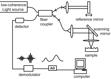
The early OCT implementations [54], referred to as time domain (TD) systems, is implemented by an axially scanning mirror in the reference arm and detects all wavelengths simultaneously in a single element detector. A simple optical setup for a time domain OCT system utilizing a low coherence source and a Michelson-type interferometer is shown in Fig. 1.1.

scanning

mirror

low-coherence

Light source

AD

demodulator

detector

fiber

coupler

reference mirror

sample

computer

Figure 1.1: Simplified OCT system setup using a fiber based Michelson interferometer.

This system utilizes the property of low coherence interferometry: noticeable interference fringes are only generated when the path length difference is within the coherence length of the light source. The interference of the two light beams can be expressed in Eq. (1.1):

ID= [Rs+Rr] + ˆS(∆x) h

2pRsRrcos(2∆xk0)

i

(1.1)

where ∆xis the path length difference between reference and sample reflection locations;IDis the

power received at the detector;RsandRrare the power for sample and reference arm respectively;

ˆ

(18)

interference at the beam combiner. Thus, the output intensity, the interferograms can be measured and recorded as ∆xgets scanned. This would actually generate an auto-correlation if in a symmetric interferometer. The amplitude of the envelope varies for different path length differences, while the peak of the envelope occurs at path length matching (zero path length difference). If, otherwise, a coherent light source with long coherent length is used, the back-reflected beams will always interfere and generate an interferogram with constant amplitude. This would have revoked the ability of ranging the reflection location within the sample.

As mentioned above, when a low coherent light source is used, the interference fringes emerges onlywhen the reference and sample path lengths were matched to within the coherence length of the source. The coherence length, lc = 2 ln 2λ2/(π∆λ), which is inversely proportional to the spectral

bandwidth of the source, determines the axial resolution. One unique feature of this method is that this axial resolution is decoupled from the lateral resolution, which is otherwise determined by the sample arm collection optics.

1.2.2

Frequency domain OCT

In recent years, a new type of OCT imaging method - frequency domain OCT (FDOCT) [55, 56], also referred as Fourier domain OCT, spectral domain OCT (SDOCT) or spectral radar [57], has attracted a huge increase in attention due to significant benefit for actual biomedical application. In fact, the idea of Fourier domain OCT techniques can be traced back in 1995 [58], but the advantage of the Fourier domain technique was not broadly accepted and exploited until nearly a decade later. In 2003, several works almost simultaneously demonstrated FDOCT has several orders of magnitude improvement in system sensitivity, which includes theoretical calculation [59–61] and experimental results [62–64]. The clinical impact of this breakthrough was phenomenal because the significantly faster imaging speeds made imaging over very large tissue volume possible [65].

In Fourier domain OCT, the broadband interference is obtained by encoding the optical frequency with a spectrally scanning source or with a dispersive detector. It calculates the delay time by a Fourier transform of the interference spectrum of the light. The implementation of FDOCT is simple as the reference mirror is now immobilized. The acquired signal can be written as a function of frequency/wavenumber2 and path length difference in Eq. (1.2).

ID= [Rs+Rr] + ˆS(∆x) h

2pRsRrcos(2∆x∆k) i

(1.2)

where ∆kis the wavenumber difference from the center wavenumber k. Eq. (1.2) is similar to Eq. (1.1) except ∆k. One can realize that the period of the spectral oscillation of the acquired signal inkspace is proportional to the path length difference ∆x. A reflection comes from a location with

(19)

shorter path length difference will produce a spectral oscillation with a frequency lower than that of a longer one. Hence, a Fourier transform of the spectral fringes will result in a depth profile similar to that acquried from TDOCT. A typical FDOCT system can have a signal to noise ratio (SNR) of more than 110dB.

In time domain OCT, interferometric fringes are acquried by rapidly translating the reference reflector. The imaging speed is limited by the mechanical actuating of the reference mirror, which is typically below 16kHz. In contrast, Fourier domain OCT avoids the mechanical scanning of the reference arm and acquires all the reflected light from the sample simultaneously. As shown in Eq. (1.2), the optical path length difference between the scatters within sample and the reference reflections is now encoded by the frequency of the interferometric fringes. As implied in Eq. (1.2), signal resulting from all reflection can be acquired simultaneously as they are represented by different spectral oscillation frequencies. This way the reflection signal from any depth of the sample can be collected over the entire measurement time T. Therefor, FDOCT systems are intrinsically more sensitive than TDOCT systems. The SNRs for TDOCT and SDOCT can be compared for the same detector responsitivity, acquisition time, and depth scan range [59–61], as expressed in Eq. (1.3).







SNRT D = _eNρTPs0Rs SNRF D = ρT₂_ePs0Rs

(1.3)

where Ps0 is the sample arm power if the sample is fully reflective, Rs is the same sample reflectivity for both systems,ρis the detector responsivity,eis the electron charge,N is the number of channels. From Eq. (1.3), one can clearly see the sensitive advantage of a FDOCT system over a TDOCT system is about a factor ofN/2.

Depending on encoding the spectrum as a function of space or time, there are two varieties of FDOCT: 1) spectrometer based system [], where a grating is deployed to disperse the broadband light across a detector array, and 2) swept source OCT, also known as wavelength tuning interferometry (WTI) [66],optical frequency domain reflectometry (OFDR) [67], and optical frequency domain imaging (OFDI) [64], which uses a narrowband source rapidly tuned over a broad bandwidth to measure spectral oscillations in time with a high speed detector.

Spectral domain (SD) OCT

Spectral domain (SD) OCT [7] extracts spectral information by using a dispersive element to dis-tributing different optical frequencies onto a detector stripe likelikes an array-type detector (Figure 2(a)). Therefore the information of the full depth scan is available within a single exposure.

(20)

disadvantage of SD-OCT reduces its ability to imaging of deep internal locations.

Swept source (SS) OCT

Swept source (SS) OCT [8] (Figure 1-2 (b)) uses a frequency tuneabletunable laser and a point source detector. It tries aims to combine some of the advantages of standard Time domain technique and Spectral domain OCT. For operation, the laser is rapidly swept across its frequency range for each sample location. Its detector records the interrference at each wavelength individually and encodes the spectrum as a function of time.

Compared to Spectral Domain OCT technology, Swept Source OCT does not suffer from inherent sensitivity degradation at longer imaging depths. Therefore, these systems are the preferred choice where long imaging depths are desired. One of the main drawbacks of the technique are is the nonlinearities in the wavelength scanning, especially at high scanning frequencies. Another main drawback is its limited axial range. By pushing the tuning sweeping speed very high, the coherence length associated with the instantaneous line-width will suffer.

1.3

Endoscopic optical coherence tomography

(21)

single-fiber-based and may be used to create much more compact probes than other existing designs. However, depth perception is not possible in such kind of endoscopic systems.

A three-dimensional (3-D) endoscopic imaging modality that can render cross-sectional view of the internal tissue structure in the forward region ahead of the probe tip can substantially improve most forms of needle surgical procedures. This additional imaging dimension is important as it can help prevent surgical needles from perforating delicate tissue structures, such as blood vessels and nerves. In the last decade, endoscopic ultrasonography (or endosonography) has been popular among the physicians as it allows viewing real-time images of intra-abdominal organs. 2-D image slices acquired from endosonography can be manipulated to render 3-D viewing of internal structures as well. However, owing to the low spatial resolution of endoscopic ultrasound, its accuracy for imaging guided intervention, such as staging a tumor is questionable [86]. For instance, a 10 MHz, 64 element linear array, 13 mm wide ultrasound endoscopic probe offers spatial resolution of no more than 1 mm [87]. At this resolution, one can detect only moderate-sized ( 1 cm or larger in diameter) tumors. Further, we should note that smaller ultrasonic tips will render even poorer resolution. Endoscopic MRI that yields relatively higher spatial resolution compared to conventional MRI, CT, and endoscopic ultrasound, is another option for rather accurate 3-D imaging. However, large-size endoscopic MRI probes are required to achieve acceptable spatial resolution. For instance, 0.2 mm ×0.2 mm×2 mm = 0.08 mm3 voxel size could be achieved by using a large (4 cm diameter loop coil) size endoscopic MRI system [88]. Notice that in addition to the large size of endoscopic MRI, which is in centimeters, the depth resolution is still in the millimeters - this defeats the purpose of the endoscope as an interventional device.

The OCT-based endoscopes are benefit from the relative ease of performing speed and high-resolution OCT systems. In the past decades, various types of OCT probes have been design and built with the target of specific applications. The important technical characteristics for design consideration of an OCT probe include the diameter, scanning range, field of view, speed, and flexibility. Based on their scan mode, OCT probes can be divided into two groups: side-imaging and forward-imaging probes.

The big benefit of in-vivo OCT imaging is its flexible probes and endoscopes, which is uniquely suited for non-invasively accessing to various lumens of the human body such as retina, cornea, arterial plaques, and cervical, et al.

1.3.1

Side-imaging probes

(22)

side-imaging endoscopic OCT probes are suitable for imaging within a tubular organ.

1.3.2

Forward-imaging probes

In 1997, Boppart et al. reported 6.4 mm diameter lead zirconate titanate PZT cantilever-based handheld forward imaging instruments firstly [14]. Unlike side imaging OCT systems, forward-imaging OCT endoscopes [15-17] emit and collect light in front of the probe; the diameter are relatively larger than that of side-imaging imaging probes. For application, forward-imaging OCT probes are useful tool to provide tissue structural information forward of the catheter probe, such as for device placement or image-guided biopsy.

To date, most of the OCT endoscope/catheter systems are circumferential or side-scanning sys-tems (2-6). By rotating the probe orientation rapidly, a cross-sectional view of the tissue can be generated. However, forward-imaging OCT endoscopic systems would be very useful in providing tissue structural information forward of the probe tip for the purpose of surgical guidance. Unlike side-imaging OCT systems, the implementation of such a forward-imaging system within a narrow probe poses very significant technological challenges, and the narrowest forward-imaging scope re-ported to date, without using our paired-angled rotation-scan technology, has been 2.4 mm wide, too large to fit within a surgical needle (7).

1.3.3

Penetration in blood

OCT penetration through blood is limited. This fact has been noted by researchers in the field of intravascular imaging since late 90’s [89]. OCT signal attenuation by blood has been believed to be a result of the optical scattering rising from intracellular/extracellular refractive index mismatch between the cytoplasm of erythrocytes and serum for infrared light.

This belief was qualitatively verified in [90]. A reflector, as a target, was imaged by OCT in the presence of saline, blood (hematocrit [Hct], 35%), and lysed blood (Hct, 1%). As shown in Fig. 1 of the article, it was difficult to locate the reflector in presence of blood while signal intensity returned to values close to saline after the red cells were lysed. This implies that membranes or hemoglobin absorption is not the main source of near infrared attenuation by blood.

In the same work [90], OCT penetration depth in blood was investigated and quantified to be about 2mmby their experimental setup. A reflector was placed in a tubing with a diameter of 6mm. The section of reflector imaged was about 2mm below inner surface of tubing. Once blood was introduced into system and circulated, OCT imaging of reflector was performed. After compounds were introduced into blood to balance the intracellular/extracellular index, an even higher contrast was achieved due to the reduced signal attenuation by scattering.

(23)

in real blood environments as it was achieved in a saline-diluted blood with an Hct of 35%. The authors stated several reasons why they did not use fresh blood. Second, the target imaged in the test was a metal reflector. One would expect a weaker signal for biological tissues like vessel wall.

A more close to practical applications but less quantitative test was carried in [89]. The impact of blood on OCT imaging, with and without saline injections, was compared. Immediately following a saline injection, nearly the entire wall of the aorta was visible. A small portion of the front was present in the image, obstructing the view of the vessel wall behind it. The second image was taken when blood filled almost half the lumen, resulting in an inability to identify the vessel wall in this region. When no saline injection was performed, the wall could only be delineated when the catheter was in direct approximation.

The most common ways to get a clear view for OCT examination in blood environment are saline flush and balloon occlusion [91, 92].

When saline flush is applied, the time span for clear OCT imaging is about 2-3 seconds [92–94] while the volume injected per bolus is about 8-10ml [92–95]. This relatively short window allows sampling of only discrete transverse segments, precluding continuous imaging of longer sections of vessel walls [92, 93]. Another problem with saline flush is that imaging during rapid variations in saline flow might produce a “wavy” appearance of the vessel wall [89]. In addition, saline delivery through the guide catheter to displace blood was inefficient for some tissue structures [94]. Several factors that influence the effectiveness of saline flush were discussed in [94].

With proximal balloon occlusion and continuous flushing, longer segments of vessel walls can be imaged. The LightLab system utilizes low pressure (0.5 atm) proximal balloon occlusion together with distal flush from the tip of the catheter. With balloon occlusion for 35 seconds and a pull-back rate of 1 mm/second, continuous imaging of a 35 mm coronary segment is possible [92]. The disad-vantages for balloon occlusion are the relatively cumbersome configuration compared with current intra-vascular ultra-sound (IVUS) systems, possible transient ischemia in the territory of the artery under study, and some concerns about the local consequences of balloon inflation. Furthermore, inadequate displacement of blood can be a problem in vessels with a diameter of 3.5 mm or greater, where large bifurcations are present and in the presence of competitive flow from collaterals or bypass grafts [92].

A discussion on how to select the two different methods can be found in [89].

Since 1999, relying on saline flush or balloon occlusion, intravascular OCT imaging has been used to different applications, such as intra-arterial imaging [89] (1999), visualization of coronary atherosclerotic plaques [93] (2002), evaluation of intracoronary stenting [94] (2003), mechanical analysis of atherosclerotic plaques [95] (2004).

(24)

methods were summarized, including saline flush, balloon occlusion, index matching, and replace-ment of blood with optically transparent hemoglobin-based blood substitute. The later two, index matching technique [90] and transparent substitute were rarely reported. Although they are poten-tially to be a elegant way to improve the penetration, current compounds for index matching do not increase penetration sufficiently for in vivo use, as admitted by the authors [90]. In the most recent paper (Dec 2008) reviewed here [96], saline flush was still employed to get a clear view for OCT imaging in order to investigate mechanical properties of vascular tissues.

Most reported cardiac OCT practices up to now are still using saline flush or balloon occlusion. Some other mitigation techniques have been investigated, such as index matching. Although appear to be promising, their practical applications haven’t been reported yet.

(25)

References

[1] G. T. Herman, Fundamentals of Computerized Tomography: Image Reconstruction from Pro-jections. Springer, 2009, p. 297 (cit. on p. 1).

[2] D. L. Bailey, D. W. Townsend, P. E. Valk, and M. N. Maisey, Eds., Positron Emission To-mography: Basic Sciences. Springer, 2005, p. 392 (cit. on p. 1).

[3] S. C. Richard, Foundations of Biomedical Ultrasound. Oxford University Press, 2006, p. 832 (cit. on p. 1).

[4] R. H. Hashemi, M.D., W. G. Bradley, Jr., and C. J. Lisanti, MRI: The Basics. Lippincott Williams & Wilkins, 2010, p. 385 (cit. on p. 1).

[5] K. T. Foley and M. M. Smith, “Image-guided spine surgery.,” Neurosurgery clinics of North America, vol. 7, no. 2, pp. 171–86, Apr. 1996 (cit. on p. 1).

[6] R. D. Bucholz, K. R. Smith, K. A. Laycock, and L. L. McDurmont, “Three-dimensional lo-calization: from image-guided surgery to information-guided therapy.,” Methods (San Diego, Calif.), vol. 25, no. 2, pp. 186–200, Oct. 2001 (cit. on p. 1).

[7] R. Ewers, K. Schicho, M. Truppe, R. Seemann, A. Reichwein, M. Figl, and A. Wagner, “Computer-aided navigation in dental implantology: 7 years of clinical experience.,” Jour-nal of oral and maxillofacial surgery : official jourJour-nal of the American Association of Oral and Maxillofacial Surgeons, vol. 62, no. 3, pp. 329–34, Mar. 2004 (cit. on p. 1).

[8] A. H. Chan, V. Y. Fujimoto, D. E. Moore, R. T. Held, M. Paun, and S. Vaezy, “In vivo feasibil-ity of image-guided transvaginal focused ultrasound therapy for the treatment of intracavitary fibroids.,”Fertility and sterility, vol. 82, no. 3, pp. 723–30, Sep. 2004 (cit. on p. 1).

[9] J. T. Yap, J. P. J. Carney, N. C. Hall, and D. W. Townsend, “Image-guided cancer therapy using PET/CT.,” Cancer journal (Sudbury, Mass.), vol. 10, no. 4, pp. 221–33, 2004 (cit. on p. 1).

[10] J. Ricke, P. Wust, A. Stohlmann, A. Beck, C. H. Cho, M. Pech, G. Wieners, B. Spors, M. Werk, C. Rosner, E. L. H¨anninen, and R. Felix, “CT-guided interstitial brachytherapy of liver malignancies alone or in combination with thermal ablation: phase I-II results of a novel tech-nique.,”International journal of radiation oncology, biology, physics, vol. 58, no. 5, pp. 1496– 505, Apr. 2004 (cit. on p. 1).

(26)

[12] E. J. Hall and D. J. Brenner, “Cancer risks from diagnostic radiology.,” The British journal of radiology, vol. 81, no. 965, pp. 362–78, May 2008 (cit. on p. 1).

[13] J. M. Cuttler and M. Pollycove, “Nuclear energy and health: and the benefits of low-dose radiation hormesis.,”Dose-response : a publication of International Hormesis Society, vol. 7, no. 1, pp. 52–89, Jan. 2009 (cit. on p. 1).

[14] D. J. Brenner and E. J. Hall, “Computed tomography–an increasing source of radiation expo-sure.,”The New England journal of medicine, vol. 357, no. 22, pp. 2277–84, Nov. 2007 (cit. on p. 1).

[15] G. Brix, U. Lechel, G. Glatting, S. I. Ziegler, W. M¨unzing, S. P. M¨uller, and T. Beyer, “Ra-diation exposure of patients undergoing whole-body dual-modality 18F-FDG PET/CT exam-inations.,”Journal of nuclear medicine : official publication, Society of Nuclear Medicine, vol. 46, no. 4, pp. 608–13, Apr. 2005 (cit. on p. 1).

[16] D. Formica and S. Silvestri, “Biological effects of exposure to magnetic resonance imaging: an overview.,”Biomedical engineering online, vol. 3, no. 1, p. 11, Apr. 2004 (cit. on p. 1).

[17] (UCSF Medical Center), Magnetic resonance safety policy of UCSF (cit. on p. 2).

[18] M. S. Cohen, R. M. Weisskoff, R. R. Rzedzian, and H. L. Kantor, “Sensory stimulation by time-varying magnetic fields.,”Magnetic resonance in medicine : official journal of the Society of Magnetic Resonance in Medicine / Society of Magnetic Resonance in Medicine, vol. 14, no. 2, pp. 409–14, May 1990 (cit. on p. 2).

[19] T. F. Budinger, H. Fischer, D. Hentschel, H. E. Reinfelder, and F. Schmitt, “Physiological effects of fast oscillating magnetic field gradients.,”Journal of computer assisted tomography, vol. 15, no. 6, pp. 909–14, 1991 (cit. on p. 2).

[20] M. Berger, M. K. Gould, and P. G. Barnett, “The cost of positron emission tomography in six United States Veterans Affairs hospitals and two academic medical centers.,”AJR. American journal of roentgenology, vol. 181, no. 2, pp. 359–65, Aug. 2003 (cit. on p. 2).

[21] A. Siemens,SOMATOM Definition Edge (cit. on p. 2).

[22] ——,MAGNETOM Trio, A Tim System (cit. on p. 2).

[23] G. e. d´ıaz,Ultrasound Physics : Main differences between Ultrasound and X-rays(cit. on p. 2).

[24] L. A. Bappa and I. A. Yakasai, “Colposcopy: The scientific basis.,”Annals of African medicine, vol. 12, no. 2, pp. 86–9, 2013 (cit. on p. 2).

(27)

[26] J. Ren, H. K. Gille, J. Wu, and C. Yang, “Ex vivo optical coherence tomography imaging of collector channels with a scanning endoscopic probe.,” Investigative ophthalmology & visual science, vol. 52, no. 7, pp. 3921–5, Jun. 2011 (cit. on p. 2).

[27] J. Schmitt, S. Lee, and K. Yung, “An optical coherence microscope with enhanced resolving power in thick tissue,”Optics Communications, vol. 142, no. 4-6, pp. 203–207, Oct. 1997 (cit. on p. 2).

[28] B. Povazay, K. Bizheva, A. Unterhuber, B. Hermann, H. Sattmann, A. F. Fercher, W. Drexler, A. Apolonski, W. J. Wadsworth, J. C. Knight, P. S. J. Russell, M. Vetterlein, and E. Scherzer, “Submicrometer axial resolution optical coherence tomography,” EN,Optics Letters, vol. 27, no. 20, p. 1800, Oct. 2002 (cit. on p. 2).

[29] American National Standards Institute, Safe Use of Lasers, Orlando, Florida., 2000 (cit. on p. 3).

[30] E. A. Swanson, J. A. Izatt, M. R. Hee, D. Huang, C. P. Lin, J. S. Schuman, C. A. Puliafito, and J. G. Fujimoto, “In vivo retinal imaging by optical coherence tomography,” EN,Optics Letters, vol. 18, no. 21, p. 1864, Nov. 1993 (cit. on p. 3).

[31] J. A. Izatt, M. R. Hee, and D. Huang, “High-speed In-Vivo retinal imaging with optical coherence tomography,”Investigative ophthalmology & visual science, vol. 35, no. 4, pp. 1729– 1729, 1994 (cit. on p. 3).

[32] M. R. Hee, J. A. Izatt, and E. A. Swanson, “Optical coherence tomography of the human retina,”Archives of Ophthalmology, vol. 113, no. 3, pp. 325–332, 1995 (cit. on p. 3).

[33] A. G. Podoleanu, G. M. Dobre, D. J. Webb, and D. A. Jackson, “Simultaneous en-face imaging of two layers in the human retina by low-coherence reflectometry,” EN, Optics Letters, vol. 22, no. 13, p. 1039, Jul. 1997 (cit. on p. 3).

[34] J. F. de Boer, T. E. Milner, M. J. C. van Gemert, and J. S. Nelson, “Two-dimensional bire-fringence imaging in biological tissue by polarization-sensitive optical coherence tomography,” EN,Optics Letters, vol. 22, no. 12, p. 934, Jun. 1997 (cit. on p. 3).

[35] M. J. Everett, K. Schoenenberger, J. Colston, and L. B. Da Silva, “Birefringence character-ization of biological tissue by use of optical coherence tomography,” EN, Optics Letters, vol. 23, no. 3, p. 228, Feb. 1998 (cit. on p. 3).

(28)

[37] S. Yazdanfar, A. M. Rollins, and J. A. Izatt, “Imaging and velocimetry of the human retinal circulation with color Doppler optical coherence tomography,”Optics Letters, vol. 25, no. 19, p. 1448, Oct. 2000 (cit. on p. 3).

[38] K. D. Rao, M. A. Choma, S. Yazdanfar, A. M. Rollins, and J. A. Izatt, “Molecular contrast in optical coherence tomography by use of a pump probe technique,” EN,Optics Letters, vol. 28, no. 5, p. 340, Mar. 2003 (cit. on p. 3).

[39] C. Yang, “Molecular Contrast Optical Coherence Tomography: A Review,” Photochemistry and Photobiology, vol. 81, no. 2, p. 215, 2005 (cit. on p. 3).

[40] U. Morgner, W. Drexler, F. X. K¨artner, X. D. Li, C. Pitris, E. P. Ippen, and J. G. Fujimoto, “Spectroscopic optical coherence tomography,”Optics Letters, vol. 25, no. 2, p. 111, Jan. 2000 (cit. on p. 3).

[41] R. Leitgeb, M. Wojtkowski, A. Kowalczyk, C. K. Hitzenberger, M. Sticker, and A. F. Fercher, “Spectral measurement of absorption by spectroscopic frequency-domain optical coherence tomography,”Optics Letters, vol. 25, no. 11, p. 820, Jun. 2000 (cit. on p. 3).

[42] D. Huang, E. Swanson, C. Lin, J. Schuman, W. Stinson, W. Chang, M. Hee, T. Flotte, K. Gregory, C. Puliafito, and A. Et, “Optical coherence tomography,”Science, vol. 254, no. 5035, pp. 1178–1181, Nov. 1991 (cit. on p. 3).

[43] A. F. Fercher, C. K. Hitzenberger, W. Drexler, G. Kamp, and H. Sattmann, “In vivo optical coherence tomography.,” American journal of ophthalmology, vol. 116, no. 1, pp. 113–4, Jul. 1993 (cit. on p. 3).

[44] J. M. Schmitt, A. Kn¨uttel, M. Yadlowsky, and M. A. Eckhaus, “Optical-coherence tomogra-phy of a dense tissue: statistics of attenuation and backscattering.,” Physics in medicine and biology, vol. 39, no. 10, pp. 1705–20, Oct. 1994 (cit. on p. 3).

[45] J. G. Fujimoto, M. E. Brezinski, G. J. Tearney, S. A. Boppart, B. Bouma, M. R. Hee, J. F. Southern, and E. A. Swanson, “Optical biopsy and imaging using optical coherence tomogra-phy.,”Nature medicine, vol. 1, no. 9, pp. 970–2, Sep. 1995 (cit. on p. 3).

[46] J. Gallwas, R. Gaschler, H. Stepp, K. Friese, and C. Dannecker, “3D optical coherence to-mography of cervical intraepithelial neoplasia–early experience and some pitfalls.,” European journal of gynaecological oncology, vol. 33, no. 1, pp. 37–41, Jan. 2012 (cit. on p. 3).

(29)

[48] E. Osiac, A. S˘aftoiu, D. I. Gheonea, I. Mandrila, and R. Angelescu, “Optical coherence to-mography and Doppler optical coherence toto-mography in the gastrointestinal tract.,” World journal of gastroenterology : WJG, vol. 17, no. 1, pp. 15–20, Jan. 2011 (cit. on p. 3).

[49] H. Wang, W. Kang, H. Zhu, G. MacLennan, and A. M. Rollins, “Three-dimensional imaging of ureter with endoscopic optical coherence tomography.,”Urology, vol. 77, no. 5, pp. 1254–8, May 2011 (cit. on p. 3).

[50] G. J. Tearney, K. Jang, and B. E. Bouma, “Optical coherence tomography for imaging the vulnerable plaque.,”Journal of biomedical optics, vol. 11, no. 2, p. 021 002, 2006 (cit. on p. 3).

[51] G. J. Tearney, M. E. Brezinski, B. E. Bouma, S. A. Boppart, C. Pitris, J. F. Southern, and J. G. Fujimoto, “In vivo endoscopic optical biopsy with optical coherence tomography.,” Science (New York, N.Y.), vol. 276, no. 5321, pp. 2037–9, Jun. 1997 (cit. on p. 3).

[52] L. Liu, J. A. Gardecki, S. K. Nadkarni, J. D. Toussaint, Y. Yagi, B. E. Bouma, and G. J. Tearney, “Imaging the subcellular structure of human coronary atherosclerosis using micro-optical coherence tomography.,”Nature medicine, vol. 17, no. 8, pp. 1010–4, Aug. 2011 (cit. on p. 4).

[53] H. Liang, M. Sax, D. Saunders, and M. Tite, “Optical Coherence Tomography for the non-invasive investigation of the microstructure of ancient Egyptian faience,”Journal of Archaeo-logical Science, vol. 39, no. 12, pp. 3683–3690, Dec. 2012 (cit. on p. 4).

[54] J. Schmitt, “Optical coherence tomography (OCT): a review,”IEEE Journal of Selected Topics in Quantum Electronics, vol. 5, no. 4, pp. 1205–1215, 1999 (cit. on p. 5).

[55] M. Wojtkowski, R. Leitgeb, A. Kowalczyk, T. Bajraszewski, and A. F. Fercher, “In vivo hu-man retinal imaging by Fourier domain optical coherence tomography.,”Journal of biomedical optics, vol. 7, no. 3, pp. 457–63, Jul. 2002 (cit. on p. 6).

[56] M. Wojtkowski, V. J. Srinivasan, T. H. Ko, J. G. Fujimoto, A. Kowalczyk, and J. S. Duker, “Ultrahigh-resolution, high-speed, Fourier domain optical coherence tomography and methods for dispersion compensation,”Optics Express, vol. 12, no. 11, p. 2404, May 2004 (cit. on p. 6).

[57] G. Ha Usler and M. W. Lindner, “”Coherence radar” and ”spectral radar”-new tools for dermatological diagnosis.,” Journal of biomedical optics, vol. 3, no. 1, pp. 21–31, Jan. 1998 (cit. on p. 6).

(30)

[59] M. Choma, M. Sarunic, C. Yang, and J. Izatt, “Sensitivity advantage of swept source and Fourier domain optical coherence tomography,” EN,Optics Express, vol. 11, no. 18, p. 2183, Sep. 2003 (cit. on pp. 6, 7).

[60] J. F. de Boer, B. Cense, B. H. Park, M. C. Pierce, G. J. Tearney, and B. E. Bouma, “Im-proved signal-to-noise ratio in spectral-domain compared with time-domain optical coherence tomography,” EN,Optics Letters, vol. 28, no. 21, p. 2067, Nov. 2003 (cit. on pp. 6, 7).

[61] R. Leitgeb, C. Hitzenberger, and A. Fercher, “Performance of fourier domain vs time domain optical coherence tomography,” EN,Optics Express, vol. 11, no. 8, p. 889, Apr. 2003 (cit. on pp. 6, 7).

[62] M. Wojtkowski, T. Bajraszewski, P. Targowski, and A. Kowalczyk, “Real-time in vivo imaging by high-speed spectral optical coherence tomography,” EN, Optics Letters, vol. 28, no. 19, p. 1745, Oct. 2003 (cit. on p. 6).

[63] S. Yun, G. Tearney, B. Bouma, B. Park, and J. de Boer, “High-speed spectral-domain optical coherence tomography at 13 µm wavelength,” EN, Optics Express, vol. 11, no. 26, p. 3598, Dec. 2003 (cit. on p. 6).

[64] S. Yun, G. Tearney, J. de Boer, N. Iftimia, and B. Bouma, “High-speed optical frequency-domain imaging,” EN,Optics Express, vol. 11, no. 22, p. 2953, Nov. 2003 (cit. on pp. 6, 7).

[65] S. H. Yun, G. J. Tearney, B. J. Vakoc, M. Shishkov, W. Y. Oh, A. E. Desjardins, M. J. Suter, R. C. Chan, J. A. Evans, K. Jang, N. S. Nishioka, J. F. de Boer, and B. E. Bouma, “Comprehensive volumetric optical microscopy in vivo.,” Nature medicine, vol. 12, no. 12, pp. 1429–33, Dec. 2006 (cit. on p. 6).

[66] F. Lexer, C. K. Hitzenberger, A. F. Fercher, and M. Kulhavy, “Wavelength-tuning interfer-ometry of intraocular distances,” Applied Optics, vol. 36, no. 25, p. 6548, Sep. 1997 (cit. on p. 7).

[67] B. Golubovic, B. E. Bouma, G. J. Tearney, and J. G. Fujimoto, “Optical frequency-domain reflectometry using rapid wavelength tuning of a Crˆ4+:forsterite laser,” Optics Letters, vol. 22, no. 22, p. 1704, Nov. 1997 (cit. on p. 7).

[68] Kelling and G, “Endoscopy of the oesophagus and stomach,” Lancet, vol. 1, pp. 1189–1198, 1900 (cit. on p. 8).

[69] Killian and G, “On direct endoscopy of the upper air passages and oesophagus : Its diagnostic and therapeutic value in the search for and removal of foreign bodies,”British Medical Journal, vol. 1902, pp. 569–571, 1902 (cit. on p. 8).

(31)

[71] S. Lam, C. MacAulay, J. C. LeRiche, and B. Palcic, “Detection and localization of early lung cancer by fluorescence bronchoscopy.,”Cancer, vol. 89, no. 11 Suppl, pp. 2468–73, Dec. 2000 (cit. on p. 8).

[72] Schindler and R, “Gastroscopy,”Lancet, vol. 1, pp. 1361–1361, 1938 (cit. on p. 8).

[73] D. C. Cumberland, “Fibre-optic endoscopy and radiology in the investigation of the ipper gastrointestinatract.,” Clinical radiology, vol. 26, no. 2, pp. 223–36, Apr. 1975 (cit. on p. 8). [74] H. Zeng, A. Weiss, R. Cline, and C. E. MacAulay, “Real-time endoscopic fluorescence imaging

for early cancer detection in the gastrointestinal tract,”Bioimaging, vol. 6, no. 4, pp. 151–165, Dec. 1998 (cit. on p. 8).

[75] J. D. Rogge, M. F. Elmore, S. J. Mahoney, E. D. Brown, F. P. Troiano, D. R. Wagner, D. J. Black, and D. C. Pound, “Low-cost, office-based, screening colonoscopy.,”The American journal of gastroenterology, vol. 89, no. 10, pp. 1775–80, Oct. 1994 (cit. on p. 8).

[76] A. D. M¨uller and A. Sonnenberg, “Protection by endoscopy against death from colorectal cancer. A case-control study among veterans.,”Archives of internal medicine, vol. 155, no. 16, pp. 1741–8, Sep. 1995 (cit. on p. 8).

[77] D. K. Rex, “Colonoscopy: a review of its yield for cancers and adenomas by indication.,”The American journal of gastroenterology, vol. 90, no. 3, pp. 353–65, Mar. 1995 (cit. on p. 8).

[78] F. C. Menken, “[Micro-endoscopy of the uterine cervix (author’s transl)].,” Geburtshilfe und Frauenheilkunde, vol. 41, no. 3, pp. 192–3, Mar. 1981 (cit. on p. 8).

[79] A. L. Magos, N. Bournas, R. Sinha, L. Lo, and R. E. Richardson, “Transvaginal endoscopic oophorectomy.,”American journal of obstetrics and gynecology, vol. 172, no. 1 Pt 1, pp. 123–4, Jan. 1995 (cit. on p. 8).

[80] J. Donnez and M. Nisolle, “Endoscopic laser treatment of uterine malformations.,” Human reproduction (Oxford, England), vol. 12, no. 7, pp. 1381–7, Jul. 1997 (cit. on p. 8).

[81] R. I. Schnall, H. M. Baer, and E. J. Seidmon, “Endoscopy for removal of unusual foreign bodies in urethra and bladder.,”Urology, vol. 34, no. 1, pp. 33–5, Jul. 1989 (cit. on p. 8).

[82] M. Grasso, M. Fraiman, and M. Levine, “Ureteropyeloscopic diagnosis and treatment of upper urinary tract urothelial malignancies.,” Urology, vol. 54, no. 2, pp. 240–6, Aug. 1999 (cit. on p. 8).

[83] L. S. Marks, “Serial endoscopy following visual laser ablation of prostate (VLAP),” Urology, vol. 42, no. 1, pp. 66–71, Jul. 1993 (cit. on p. 8).

(32)

[85] G. J. Tearney, M. Shishkov, and B. E. Bouma, “Spectrally encoded miniature endoscopy.,” Optics letters, vol. 27, no. 6, pp. 412–4, Mar. 2002 (cit. on p. 8).

[86] J. F. Botet, C. J. Lightdale, A. G. Zauber, H. Gerdes, C. Urmacher, and M. F. Brennan, “Preoperative staging of esophageal cancer: comparison of endoscopic US and dynamic CT.,” Radiology, vol. 181, no. 2, pp. 419–25, Nov. 1991 (cit. on p. 9).

[87] E. P. Dimagno, P. T. Regan, J. E. Clain, E. M. James, and J. L. Buxton, “Human endoscopic ultrasonography.,”Gastroenterology, vol. 83, no. 4, pp. 824–9, Oct. 1982 (cit. on p. 9).

[88] I. Yamada, N. Saito, K. Takeshita, N. Yoshino, A. Tetsumura, J. Kumagai, and H. Shibuya, “Early gastric carcinoma: evaluation with high-spatial-resolution MR imaging in vitro.,” Ra-diology, vol. 220, no. 1, pp. 115–21, Jul. 2001 (cit. on p. 9).

[89] J. G. Fujimoto, S. A. Boppart, G. J. Tearney, B. E. Bouma, C. Pitris, and M. E. Brezinski, “High resolution in vivo intra-arterial imaging with optical coherence tomography.,” Heart (British Cardiac Society), vol. 82, no. 2, pp. 128–33, Aug. 1999 (cit. on pp. 10–12).

[90] M. Brezinski, K. Saunders, C. Jesser, X. Li, and J. Fujimoto, “Index matching to improve optical coherence tomography imaging through blood.,”Circulation, vol. 103, no. 15, pp. 1999– 2003, Apr. 2001 (cit. on pp. 10, 12).

[91] A. M. Zysk, F. T. Nguyen, A. L. Oldenburg, D. L. Marks, and S. A. Boppart, “Optical coherence tomography: a review of clinical development from bench to bedside.,” Journal of biomedical optics, vol. 12, no. 5, p. 051 403, 2007 (cit. on p. 11).

[92] O. C. Raffel, T. Akasaka, and I.-K. Jang, “Cardiac optical coherence tomography.,” Heart (British Cardiac Society), vol. 94, no. 9, pp. 1200–10, Sep. 2008 (cit. on p. 11).

[93] K. Jang, B. E. Bouma, D.-H. Kang, S.-J. Park, S.-W. Park, B. Seung, K.-B. Choi, M. Shishkov, K. Schlendorf, E. Pomerantsev, S. L. Houser, H. T. Aretz, and G. J. Tearney, “Visualization of coronary atherosclerotic plaques in patients using optical coherence tomography: comparison with intravascular ultrasound.,”Journal of the American College of Cardiology, vol. 39, no. 4, pp. 604–9, Feb. 2002 (cit. on p. 11).

[94] B. E. Bouma, G. J. Tearney, H. Yabushita, M. Shishkov, C. R. Kauffman, D. DeJoseph Gau-thier, B. D. MacNeill, S. L. Houser, H. T. Aretz, E. F. Halpern, and I.-K. Jang, “Evaluation of intracoronary stenting by intravascular optical coherence tomography.,”Heart (British Cardiac Society), vol. 89, no. 3, pp. 317–20, Mar. 2003 (cit. on p. 11).

(33)

(34)

Chapter 2

Optical Coherence Tomography

Probe I - Manual Scanning

Optical Coherence Tomography’s (OCT) non-invasive nature and high resolution has made it an important modality in the field of biomedical imaging since 90’s [1]. Aside from ophthalmology applications [2, 3], OCT has been implemented in various probes and endoscopic formats for various applications [4, 5]. Various methods for sweeping the OCT probe beam to accomplish scans have been developed over the years and almost all of them involve some form of mechanical actuations. While these systems allow for good scan controls and result in excellently rendered OCT images, they do come with the associated cost of additional hardware that need to be integrated well onto the probes. A hand-held OCT probe that can be manually swept over the region of interest by the user and that provides an OCT scan of the biological structures along the device’s motion trajectory, can potentially simplify the whole procedure of image acquisition.

In this chapter, we report a new OCT probe design based on position tracking to achieve the above manual-scanning capability. We developed an optical monitoring system can continuously track the position and orientation (henceforth referred to as the pose) of a simple OCT probe while the probe is manually scanned over a region of interest. Both planar 2D images and volumetric 3D images could be reconstructed by orienting each OCT depth scan (A-scan) according to their individual spatial location and direction as resolved from the poses of the hand-held device. Unlike mechanically actuated OCT probes that reconstruct images based on pre-determined scan patterns [6–13], this method can objectively track and measure the real scan pattern regardless of the scanning mechanism or pattern.

2.1

Hand-Held manual scanning probe by position tracking

(35)

information of the probe, that can be combined with A line data to create OCT images. This idea is illustrated in the following figure:

Figure 2.1: Illustration of mechanical and manual scanning

However, challenges are still left. As shown in Figure 2.2, non-uniformity and uncertainty of hand motion will significantly distort the acquired images since the spatial sampling of OCT axial scans can not maintain uniform. Therefore if there is not external mechanism to restore the hand motion information, one cannot recover the structure under test.

Figure 2.2: Image artifact induced by non-uniformity of hand motion.

(36)

2.2

Implementation and verification

The implemented tracking system is schematically illustrated in Figure 2.3. Four infrared LEDs centered at 950 nm were mounted on a tetrahedron frame to serve as feature points. Taking one of the LEDs as the origin of the reference frame, the coordinates for these feature points were (0, 0, 0), (43mm, 0, 0), (0, 43mm, 0), (0, 0, 43mm) respectively. An OCT needle probe was attached to this frame along the direction of (-1, -1, -1). A monochrome CMOS camera with a focal length of 25.4mm was placed about 51cm away from the hand-held probe. Its frame rate was configured at 30fps with a pixel array of 1280 by 1024. The sensor pixel size is 5.2 microns. With this optical arrangement, a plane 51 cm from the camera was recorded with a magnification factor of 0.05 and the achieved field-of-view was 13.3cm by 10.6cm. The camera captured 2D images of the feature points. The positions of these four feature points in the recorded images provide sufficient information for the determination of the probe’s pose in 3D.

Figure 2.3: Schematic of the tracking system. The left bottom inset is a photo of our prototype hand-held probe. The right top inset is a 3D rendering of the probe by the tracking system.

In the first stage of pose determination, we employ a pair of blob detector and tracker programs to locate the feature points in each image and track their correspondence among a sequence of images. We then determine each feature point’s location with sub-pixel resolution ( 0.03 pixels) by applying a centroid-based estimation algorithm in a surrounding square region after the center of the feature point has been approximately identified by the programs. The choice of the selected region size will ultimately impact on the achieved accuracy of the pose computation. Our evaluation experiments (described later in this paper) led us to choose a 21 x 21 pixel grid for optimal operation.

(37)

con-vergence. The algorithm basically applies the scaled orthographic projection (SOP) to approximate the prospective projection occurring in the camera; it simplifies the task of solving a set of nonlinear equations into iteratively solving a few sets of linear equations. The tracking system allowed us to track the probe’s pose at intervals limited only by the camera’s frame rate of 30 fps. The workflow of the system is shown below:

Figure 2.4: Workflow of the OCT tracking system

Our OCT probe consisted of a needle probe with a diameter of 1.2 mm and length of 63.5 mm. A 3 mm long 0.29 pitch GRIN lens connected to a single mode fiber via a glass ferrule was housed within this needle probe. This probe focused light at a working distance of 3.9 mm (in air) ahead of its tip with a spot size of 19 microns. The schematics of the probe is illustrated in Figure 2.5. A swept laser centered at 1310nm with a scan range of about 100nm and an average power of 8.5mW served as the OCT light source. The depth scan acquisition rate (A line rate) was 333 Hz. The sensitivity of this OCT probe was measured as 95dB. Concurrent with the pose tracking, our OCT probe continuously acquired A-scans and transferred the data into the computer.

Figure 2.5: Schematics of the hand-held probe

(38)

along the scan direction (orthogonal to the OCT probe’s main axis) in increments of 10 microns. At each location, a group of 100 images were captured as a sufficient statistical ensemble and ana-lyzed for pose estimation. For each sample image, we varied the size of the selected square regions around each identified feature point from 3 x 3 to 201 x 201 pixels during feature point centroid computations.

Figure 2.6: Tracking accuracy characterization

(39)

able to determine the position of the probe with an accuracy of 5.8 microns at the optimal window size.

The existence of a sweet spot for positional accuracy is not surprising. If we choose a window size that is overly small, we will reject some of the light contribution from the feature point from the position calculation and therefore expect to introduce errors. On the other hand, an overly large window size ensures that we fully consider all light contributions associated with the feature point; however, such a choice will also assign undue weighting on spurious background signals.

We further evaluated the probe’s tracking ability perpendicular to the scan direction (in other words, along the OCT probe’s main axis) via a similar experiment and determined that the tracking accuracy along that axis was 18.8µm.

2.3

Proof-of-Principle experiments

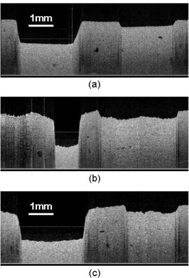
To demonstrate that this tracking approach can indeed be employed to generate reasonable OCT images, we performed a number of scans with the probe on a phantom sample. The phantom sample consisted of an agarose gel block embedded with 0.2 micron latex microspheres at 0.66% volume concentration. Two grooves were intentionally carved on its surface. They were roughly 2.5mm wide and spaced 2.2mm apart. The first groove was 1.3 mm deep and the second was 0.3 mm deep. We first translated the probe across the surface of this sample via a motorized translation stage. The collected OCT image from this scan is shown in Figure 2.7(a) and serves as the control. Next, we held the probe by hand and manually scanned the probe across the sample. This manual scan took 6 second and occurred over a length of 7.5 mm. If we simply stack the collected A-scans based on time-order, the resulting OCT image (shown in Figure 2.7(b)) corresponds poorly to our control image (Figure 2.7(a)). This is attributable to the fact that our manual scan motion exhibited significant velocity variations during the scan. In comparison, the construction of the OCT image based on accurate tracking of the probe’s position did a significantly better job at rendering an accurate OCT image (Figure 2.7(c)).

It is worth to mention that the frame rate of the camera was relatively slow compared to the A line acquisition rate thus there were about 10 A lines acquired between probe pose determination. We estimated the probe position for each A line by linear interpolation from the known probe pose-time points. This interpolation might introduce some pose errors. The rendered image in Figure 7(c) contains possible maximal interpolation-induced errors of 40 microns, which can be reduced with a camera of higher frame rate.

(40)

Figure 2.7: (a) Target phantom image by a motorized stage scanning (control group); (b) Target phantom image by manual scanning and reconstructed based on time order; (c) Target phantom image by manual scanning and reconstructed based on estimated displacement.

different shapes in the two images.

These experiments demonstrated that continuous pose tracking of an OCT probe is indeed useful as a means for accomplishing OCT image renderings. The position determination accuracy of 6 microns along two dimension and 19 microns along the third dimension in our prototype is a sufficiently good match with the associated resolution of the OCT system. Our proposed system can be improved by incorporating a faster frame-rate pose tracker to allow for more accurate pose tracking. Pose accuracy can also be potentially improved by employing multiple cameras at different angles to monitor the probe’s movement. This tracking system approach is potentially a good match with the confined work environment of the surgical suite, as the involved tracking camera can potentially be mounted on the suite’s ceiling.

(41)

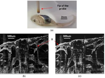
Figure 2.8: ((a) Photo of a 54 stage Xenopus Laevis tadpole specimen and the scanning probe’s tip; (b) OCT image acquired by manually scanning without tracking correction; (c) OCT image acquired by manually scanning with tracking correction; g, gill pockets.

(42)

References

[1] D. Huang, E. Swanson, C. Lin, J. Schuman, W. Stinson, W. Chang, M. Hee, T. Flotte, K. Gregory, C. Puliafito, and A. Et, “Optical coherence tomography,”Science, vol. 254, no. 5035, pp. 1178–1181, Nov. 1991 (cit. on p. 22).

[2] B. Povazay, K. Bizheva, B. Hermann, A. Unterhuber, H. Sattmann, A. Fercher, W. Drexler, C. Schubert, P. Ahnelt, M. Mei, R. Holzwarth, W. Wadsworth, J. Knight, and P. S. J. Russell, “Enhanced visualization of choroidal vessels using ultrahigh resolution ophthalmic OCT at 1050 nm,” EN,Optics Express, vol. 11, no. 17, p. 1980, Aug. 2003 (cit. on p. 22).

[3] S. Han, M. V. Sarunic, J. Wu, M. Humayun, and C. Yang, “Handheld forward-imaging needle endoscope for ophthalmic optical coherence tomography inspection.,” Journal of biomedical optics, vol. 13, no. 2, p. 020 505, Jan. 2008 (cit. on p. 22).

[4] M. V. Sivak, K. Kobayashi, J. A. Izatt, A. M. Rollins, R. Ung-Runyawee, A. Chak, R. C. Wong, G. A. Isenberg, and J. Willis, “High-resolution endoscopic imaging of the GI tract using optical coherence tomography.,”Gastrointestinal endoscopy, vol. 51, no. 4 Pt 1, pp. 474–9, Apr. 2000 (cit. on p. 22).

[5] B. E. Bouma, G. J. Tearney, H. Yabushita, M. Shishkov, C. R. Kauffman, D. DeJoseph Gau-thier, B. D. MacNeill, S. L. Houser, H. T. Aretz, E. F. Halpern, and I.-K. Jang, “Evaluation of intracoronary stenting by intravascular optical coherence tomography.,”Heart (British Cardiac Society), vol. 89, no. 3, pp. 317–20, Mar. 2003 (cit. on p. 22).

[6] G. J. Tearney, S. A. Boppart, B. E. Bouma, M. E. Brezinski, N. J. Weissman, J. F. Southern, and J. G. Fujimoto, “Scanning single-mode fiber optic catheter-endoscope for optical coherence tomography,”Optics Letters, vol. 21, no. 7, p. 543, Apr. 1996 (cit. on p. 22).

[7] X. Li, C. Chudoba, T. Ko, C. Pitris, and J. G. Fujimoto, “Imaging needle for optical coherence tomography,”Optics Letters, vol. 25, no. 20, p. 1520, Oct. 2000 (cit. on p. 22).

[8] P. R. Herz, Y. Chen, A. D. Aguirre, K. Schneider, P. Hsiung, J. G. Fujimoto, K. Madden, J. Schmitt, J. Goodnow, and C. Petersen, “Micromotor endoscope catheter for in vivo, ultrahigh-resolution optical coherence tomography,”Optics Letters, vol. 29, no. 19, p. 2261, Oct. 2004 (cit. on p. 22).

[9] J. Su, J. Zhang, L. Yu, and Z. Chen, “In vivo three-dimensional microelectromechanical endo-scopic swept source optical coherence tomography,”Optics Express, vol. 15, no. 16, p. 10 390, Aug. 2007 (cit. on p. 22).

(43)

[11] X. Liu, M. J. Cobb, Y. Chen, M. B. Kimmey, and X. Li, “Rapid-scanning forward-imaging miniature endoscope for real-time optical coherence tomography,”Optics Letters, vol. 29, no. 15, p. 1763, Aug. 2004 (cit. on p. 22).

[12] T. Xie, S. Guo, Z. Chen, D. Mukai, and M. Brenner, “GRIN lens rod based probe for en-doscopic spectral domain optical coherence tomography with fast dynamic focus tracking,” Optics Express, vol. 14, no. 8, p. 3238, Apr. 2006 (cit. on p. 22).

[13] J. Wu, M. Conry, C. Gu, F. Wang, Z. Yaqoob, and C. Yang, “Paired-angle-rotation scanning optical coherence tomography forward-imaging probe,”Optics Letters, vol. 31, no. 9, p. 1265, May 2006 (cit. on p. 22).

(44)

Chapter 3

Optical Coherence Tomography

Probe II - Mechanical Scanning

This chapter is to present some continuing improvement on Paired-Angle-Rotation Scanning (PARS) forward-imaging probe [1–3]. These include a more precise theoretical modeling of the scanning and a new design of 21/23 gauge hand-held probe. We will start with a short review on the PARS technology.

3.1

Paired-Angle-Rotation Scanning (PARS) Forward-Imaging

Probe

Forward-imaging OCT endoscopic systems can be very useful in providing tissue structural infor-mation forward of the probe tip for the purpose of surgery guidance. Unlike side-imaging OCT systems, the implementation of s