R E S E A R C H
Open Access
Goertzel algorithm generalized to non-integer
multiples of fundamental frequency
Petr Sysel and Pavel Rajmic
*Abstract
The article deals with the Goertzel algorithm, used to establish the modulus and phase of harmonic components of a signal. The advantages of the Goertzel approach over the DFT and the FFT in cases of a few harmonics of interest are highlighted, with the article providing deeper and more accurate analysis than can be found in the literature, including the memory complexity. But the main emphasis is placed on the generalization of the Goertzel algorithm, which allows us to use it also for frequencies which are not integer multiples of the fundamental frequency. Such an algorithm is derived at the cost of negligibly increasing the computational and memory complexity.
Keywords:Goertzel algorithm, generalization, spectrum, DFT, DTFT, DTMF
1 Introduction
In the case of discrete-time signals, the discrete Fourier transform (DFT) is widely used for spectral analysis. The frequencies of the harmonics in the DFT always depend on the length of the transform,N, and they are integer multiples of the fundamental frequency f = fs
N,wherefs represents the sampling frequency.
Thus, Δfgives the frequency resolution of the DFT. In the case, when the transform lengthNis not a multiple of the signal period, the signal is a sum of harmonic components whose frequencies are not integral multi-ples of the fundamental frequency. Such components
are not expressible in the N-point DFT spectrum by a
single spectral line—this effect is called “leakage” into the neighboring DFT spectral coefficients, placed at the integer multiples ofΔf[1].
Therefore, the transform lengthNalways needs to be chosen with respect to the desired accuracy of the fre-quency resolution. The computational complexity of the DFT increases quadratically with the number of sam-ples/frequencies, and thus in practice we use almost exclusively the fast Fourier transform algorithm (FFT), whose computational complexity is linearithmic (linear-logarithmic). When the task is to identify the modulus
and/or phase of a single or of just a few of the fre-quency components, even the FFT is of no advantage, because it always computes all the frequency compo-nents, most of which are discarded, as being of no inter-est. In such situations, methods specialized in computing a subset of output frequencies can be exploited with great benefit. Besides the Goertzel algo-rithm, which deals with single frequencies separately, it is worth mentioning the so-called pruned-FFT [2,3], which is also connected to the zoom-FFT algorithm [1], and the transform decomposition of Sorensen and Bur-rus [3], which efficiently combines the ideas of the split-radix FFT and the Goertzel approach. However, the essential disadvantage of rounding frequencies to the nearest integer multiples (and the inaccuracy thus intro-duced) remains if using any of these methods, including the classical version of the Goertzel algorithm.
In Section 2, we first show the derivation of the com-mon Goertzel algorithm in detail. While this may seem superfluous, it will be necessary to refer back to a num-ber of its particular steps in the later sections. Then the computational and memory complexity of the Goertzel algorithm and the FFT is compared. In Section 3, we provide the announced generalization of the Goertzel algorithm, so that it is possible to use it also for the non-integral multiples of the fundamental frequency. Such a generalization has been mentioned before, e.g., * Correspondence: [email protected]
Department of Telecommunications, Faculty of Electrical Engineering and Communication, Brno University of Technology, Purkyňova 118, 612 00 Brno, Czech Republic
in [4,1], but just for the computation of the modulus, not the phase of a harmonic component.
1.1 Example of utilization of Goertzel algorithm—DTMF
The Goertzel algorithm is typically used for frequency detection in the telephone tone dialing (dual-tone multi-frequency, DTMF), where the meaning of the signaling is determined by two out of a total of eight frequencies being simultaneously present [5]. The frequencies of each of the two groups of four signaling tones were cho-sen such that the frequencies of their higher harmonics or intermodulation products were sufficiently distant. The frequencies chosen for the DTFM have a big least common multiple. Hence, using a digital receiver with a sampling frequency of 8 kHz, the period of DTMF sig-nal amounts to several tens of thousands of samples. In
practice, however, the transform length N must be
much smaller, so naturally the effect of spectrum leak-age will appear. For example, with N= 205, instead of the accurate frequency 770 Hz the modulus at approxi-mately 780.5 Hz (= 20·8000/205) is computed. This situation is illustrated in Figure 1, where it is evident that the maximum occurs at the non-integer multiple of the fundamental frequency.
The value N = 205 is often used in practice [6],
because one of the local minima of the sum of squared relative deviations of the signaling frequencies is experi-enced precisely for this length. In this situation, the deviation is approximately equal to 1.4%, while the transmitter frequency tolerance is 1.8%. Nevertheless, in some applications of the Goertzel algorithm the devia-tion from the exact frequency can exceed a prescribed tolerance, and thus both the DFT and the Goertzel algo-rithm would be of little use.
Using the approach presented in this article it is not necessary to round the frequencies at which detection is desired; it is possible to determine the modulus and
phase of a component at an arbitrary (even non-integer) frequency. The number of operations and memory requirements increases only negligibly with this approach.
1.2 Notation
In the following text, we assume a discrete signal x of length N, whose samples can be complex, {x[n]} = {x[0], x[1],..., x[N - 1]}. Symbol k represents the number
(index) of the harmonic component in the DFT, thusk
Î N. However, in the later parts of the text, we will work also withk Î ℝ. The unit step signal is denoted by {u[n]}, whilstu[n] = 1 forn≥0,u[n] = 0 forn< 0.
2 Standard Goertzel algorithm
2.1 Derivation of standard Goertzel algorithm
The algorithm invented by Goertzel [7] serves to com-pute the kth DFT component of the signal {x[n]} of lengthN, i.e.,
X[k] =
N−1
n=0
x[n]e−j2πkNn, k= 0,. . .,N−1. (1)
Multiplying the right side of this equation by
1 = ej2πkNN leads to its equivalent
X[k] = ej2πkNN N−1
n=0
x[n]e−j2πkNn, (2)
which can be rearranged into
X[k] =
N−1
n=0
x[n]e−j2πk n−N
N . (3)
The right side of (3) can be understood as a discrete linear convolution of signals {x[n]} and {hk[n]}, provided
0 20 40 60 80 100 120 140 160 180 200 −1.5
−1 −0.5 0 0.5 1 1.5
time [samples]
0 0.005 0.01 0.015 0.02 0.025 time [s]
17.50 18 18.5 19 19.5 20 20.5 21 21.5 22 22.5 23 20
40 60 80 100
harmonics
module
17.5 18 18.5 19 19.5 20 20.5 21 21.5 22 22.5 23
−3
−2
−1 0 1 2 3
harmonics
phase
700 720 740 760 780 800 820 840 860 880 frequency [Hz]
700 720 740 760 780 800 820 840 860 880 frequency [Hz]
that the elements of the latter signal are defined by
hk[] = ej2πk
Nu[].In fact, if {yk[n]} denotes the result of such a convolution, then it holds for its entries:
yk[m] =
∞
n=−∞
x[n]hk[m−n], (4)
which can be rewritten as
yk[m] = N−1
n=0
x[n]ej2πkmN−nu[m−n] (5)
where the compact support of the signal {x[n]} is taken into consideration.
Comparing (3) and (5), it is clear that the desiredX[k] is theNth sample of the convolution, i.e.,
X[k] =yk[N] (6)
for an arbitrary but fixed k= 0,...,N- 1. This means that the required value can be obtained as the output
sample in time N of an IIR linear system with the
impulse response {hk[n]}.
The transfer functionHk(z) of this system will now be derived; it is theL-transform of its impulse response [8], thus
Hk(z) =
∞
n=−∞
hk[n]z−n (7)
=
∞
n=−∞
ej2πkNnu[n]z−n (8)
=
∞
n=0
ej2πkNnz−n (9)
=
∞
n=0
(ej2πNkz−1) n
, (10)
which can be viewed as a geometric series with the first term being equal to ej2πkN0
z−0= 1and with the quotient q= ej2πNk
z−1.For |q| < 1, i.e., |z| > 1, the ser-ies is convergent and its sum equals the desired transfer function:
Hk(z) =
1
1−ej2Nπkz−1
. (11)
The corresponding difference equation is
yk[n] =x[n] + ej2Nπkyk[n−1], withyk[−1] = 0. (12)
This first order difference equation contains a com-plex multiplication factor, which is computationally demanding. To save the computational cost, the trans-mission function can be extended in both the numerator
and the denominator by the conjugate of
(1−ej2Nπkz−1), which leads to
Hk(z) =
1−e−j2Nπkz−1
1−e−j2Nπkz−1 1−ej2πNkz−1
(13)
= 1−e
−j2πNk z−1
1−2 cos
2πk N
z−1+z−2
. (14)
The respective difference equation of this second order IIR system is
yk[n] =x[n]−x[n−1]e−j
2πk N + 2 cos
2πk
N
yk[n−1]−yk[n−2] (15)
withx[-1] =y[-1] =y[-2] = 0. Such a structure can be described using the state variables:
s[n] =x[n] + 2 cos
2πk N
s[n−1]−s[n−2], (16)
while the output is given by
yk[n] =s[n]−e−j
2πk
N s[n−1] (17)
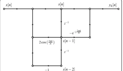
and we set s[-1] = s[-2] = 0. The signal flow graph representing the system is depicted in Figure 2.
The state-space description is advantageous because only the output sampley[N] is of interest. The algorithm iterates the real-number-only system (16) for (N+ 1) times (beginning with the sample with the time index 0; in the last iteration the input samplex[N] is put equal to
x[n] s[n] yk[n]
z−1
−e−j 2πNk
2cos2πk N
s[n−1]
z−1
−1 s[n−2]
zero). Only in the last step is the outputyk[N] calculated according to (17) using only a single complex multiplica-tion. As mentioned earlier, the value in yk[N] is the desired spectral coefficientX[k].
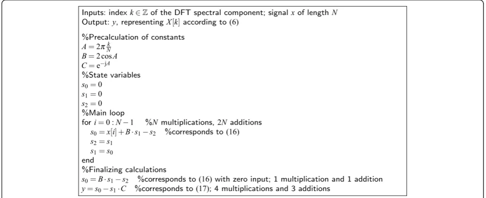
The Goertzel algorithm can hence be considered as an IIR filtering process, while only a single output sample is of interest. The algorithm is presented step by step in Figure 3.
2.2 Comparison of Goertzel algorithm and FFT
2.2.1 Properties
The Goertzel algorithm in fact performs the computa-tion of a single DFT coefficient. Compared to the DFT, it has several advantages, because of which it is used.
- First of all, the Goertzel algorithm is advantageous in situations when only values of a few spectral com-ponents are required (as in the DTMF example in Section 1.1), not the whole spectrum. In such a case the algorithm can be significantly faster.
- The efficiency of using the FFT algorithm for the computation of DFT components is strongly
deter-mined by the signal length N. The most effective
case is when Nis a power of two. On the contrary,
Ncan be arbitrary in the case of the Goertzel algo-rithm, and the computational complexity does not vary.
- The computation can be initiated at an arbitrary moment, even at the very time of the arrival of the very first input sample; it is not necessary to wait for the whole data block as in the case of the FFT. Thus, the Goertzel algorithm can be less demanding from the viewpoint of the memory capacity and it can per-form at a very low latency. Also, the Goertzel
algorithm does not need any reordering of input or output data in the bit-reverse order [1].
- Finally, as will be shown later in the article, the modulus and phase can be established also for the non-integral spectral indexesk, raising the computa-tional effort only negligibly. Therefore the Goertzel algorithm is convenient in cases when, for some rea-son, it is required to detect harmonic signals of non-integral frequencies, or, signals with a limited num-ber of samples which causes a decrease of the DFT frequency resolution.
2.2.2 Computational and memory complexities
In the following analysis, operations which can be per-formed before the first data sample has been received are not considered. Specifically, the constantsA,B,Cin Figure 3 can be precomputed. The memory performance is handled in a minimalist scenario, i.e., such that it would not be possible to implement the algorithm with fewer sto-rage locations.
The FFT algorithm used withNbeing a power of two
has computational demands proportional toNlog2N, the absolute number depends on the particular implementa-tion. Usually the number of real-number operations found in the literature is approximately 6Nlog2N(taking one complex multiplication as a combination of four multipli-cations and two summations). When working with real signals, a number of operations can be avoided; however, it is at the cost of increased complexity of the algorithm, and, it is not true that the demands can be reduced by half, as can be read, for example in [9]. For this reason, we consider the standard“complex”FFT even for real signals.
If we analyze the number of operations of the stan-dard Goertzel algorithm, we realize that for a real input
Inputs: indexk∈Zof the DFT spectral component; signalxof lengthN Output:y, representingX[k]according to(6)
%Precalculation of constants A=2πk
N B=2 cosA C=e−jA %State variables s0=0
s1=0
s2=0
%Main loop
fori=0 :N−1 %Nmultiplications,2Nadditions s0=x[i] +B·s1−s2 %corresponds to(16) s2=s1
s1=s0
end
%Finalizing calculations
s0=B·s1−s2 %corresponds to(16)with zero input; 1 multiplication and 1 addition y=s0−s1·C %corresponds to(17); 4 multiplications and 3 additions
signal, Nreal multiplications and 2Nreal additions are performed in the main loop. So the total number of operations is approximately 3Nfor a single frequency; we omit the small number of operations needed for
pre-computing B= 2 cos2Nπk,C= e−j2Nπk and the
conclud-ing complex multiplication (one for each frequencyk). Thus, ifNfrequencies were of interest, the Goertzel algo-rithm would be of quadratic complexity as the DFT is.
To answer the question“for how many frequenciesK
is it more advantageous to exploit the Goertzel
algo-rithm than the FFT” we compare
3NK<6Nlog2N
K<2log2N, (18)
which represents a more accurate result than for example [[8], p. 635], where the sharper inequalityK< log2 N, based solely on a comparison of the order of magnitude, is presented. Such a result, however, holds only forNbeing a power of two; otherwise the inequal-ity (18) can even be more favorable for the Goertzel algorithm.
The formula (18) says that the computation should be faster than the FFT as long as the number of frequen-cies does not exceed 2 log2 N. For example, with a
sig-nal of length N = 32 the Goertzel algorithm is
preferable if K ≤ 9. In the case ofN = 128 Goertzel
dominates over the FFT ifK≤13.
In fact, the algorithm introduced in [3] can be even more efficient than this. It combines the good properties of both the FFT and the Goertzel algorithm, producing a DFT decomposition similar to the one used in the split-radix FFT. The dominance of the algorithm of Sorensen and Burrus over the FFT is guaranteed even forK<N/2. An experimental comparison of this approach with the Goertzel algorithm showed that the Goertzel algorithm performs actually better than their algorithm whenK≤4 orK≤5 for a wide range ofN. It should be noticed, how-ever, that the algorithm from [3] has to work with a whole data block, and also the complexity being compared does not include rearrangement of the input data sequence.
Using the FFT algorithm requires a memory space of at least 2N, which contains the real and imaginary parts of signal samples. Also theNvalues of the transforma-tion kernel, sin and cos (so-called twiddle factors), are often precomputed and stored. The FFT calculation itself can be performed with no values being moved in memory (i.e., in-place), however, with regard to the impossibility of starting the computation until the last sample of a block of data is received, a buffer of at least 2Nin size must be used. In the case of real signals,N memory locations are enough. Thus, the overall FFT memory demand is 4Nfor real signals.
For each considered frequency, the Goertzel algorithm requires: locations for saving two state variables, the real constantB, the real and imaginary parts of the precom-puted C, and the real and imaginary parts of the final result. There is no need to implement input buffering, because the computation can be run as the new signal samples arrive. Similarly, the output signal can be over-written after the last sample has arrived. In many cases it will therefore not be necessary to use buffering at the output side either. The total memory complexity of the Goertzel algorithm is thus 7Kpositions.
Combining all the above together, the Goertzel algo-rithm will be less memory-demanding than the FFT if
7K < 4N
K< 4 7N.
(19)
A comparison of (19) and (18) leads to the conclusion that, if we look for a numberKfor which the Goertzel algorithm dominates over the FFT from both the mem-ory and the computational viewpoints, then: forN≥13 formula (18) is decisive, because for these Nit holds
4
7N>2log2N; on the other hand, for N Î {2,..., 12} (which is unusual in practice), the decisive formula is (19), because for these Nit holds 4
7N>2log2N; never-theless, as the difference of the right and the left sides does not exceed 2 in this case, we can conclude, with a small loss of generality, that the comparison of the effectiveness of the two algorithms can be based just on relation (18).
3 Generalized Goertzel algorithm
Formula (2) holds for integer-valuedk only. In such a case, the integer number of periods of the transforma-tion kernel, e−j2πkNn, corresponds to the signal length
N. In the case ofkÎℝ, formulas (1) and (2) are gener-ally no longer in agreement. (The period of the
transfor-mation kernel no longer corresponds to N, hence the
standard approach cannot be used.)
In Sections 3.1 and 3.2, we will generalize the algo-rithm such that it includes also the non-integral-valued multiples of the fundamental frequency. The complexity of the novel approach is analyzed in Section 3.3. And, as shown in Section 3.4, the non-integer case can be trea-ted by the standard algorithm using a small trick; how-ever, this is at the cost of increased computational effort.
3.1 Generalizing to non-integerk
X(ω) =
∞
n=−∞
x[n]e−jωn,ω∈R. (20)
With the notation ωk= 2πNkwe can write that
X(ωk) =
∞
n=−∞
x[n]e−j2πkNn (21)
=
N−1
n=0
x[n]e−j2πkNn, k,ωk∈R, (22)
where we exploited the compactness of the support of the signal {x[n]}.
The derivation of the generalized Goertzel algorithm is analog to the technique presented in Section 2. Com-pared to that, however, we extend formula (22) at the very beginning by unity in the form of
ej2πkNN ·e−j2πk N
N = 1 fork∈R, (23)
leading to
X(ωk) = ej2πk N
N ·e−j2πkNN N−1
n=0
x[n]e−j2πkNn (24)
= e−j2πkNN N−1
n=0
x[n]ej2πk N−n
N (25)
= e−j2πk
N−1
n=0
x[n]ej2πk N−n
N . (26)
Since the sum in (26) is identical to (3), the derivation of the generalized algorithm can proceed using the same steps as in Section 2.1, with one noteworthy change: the equation that characterizes the output using state vari-ables (17) will now be of the form
yk[n] =
s[n]−e−j2Nπks[n−1]
·e−j2πk. (27)
Indeed this is so, since the“correction constant”, e -j2πk
, depends only on the index of the frequency compo-nent, which remains constant throughout the
computa-tion. The complex constant is equal to one for kÎ Z,
which shows that this is indeed a generalization. In fact, the only variation compared to the standard Goertzel algorithm is the multiplication by this constant at the very end of the algorithm.
The constant e-j2πkaffects only the phase of the result, not the module. Among other things, this means that
the interest in the modules of the components with non-integer kcan be satisfied using the standard algo-rithm. Indeed, for example [4] uses it in this way. In cases when the phase plays a role (the delay of a signal is detected, for example), however, the use of this“ cor-rection constant” is necessary. A short remark can be found in [[1], p. 531], describing the possiblility of com-puting the Goertzel results also for non-integer-valued k; however, it misleads the reader in that the phase case is not distinguished at all.
3.2 Reducing number of iterations
It will be shown in this section that the last iteration of the Goertzel algorithm can be substituted by merely a single complex multiplication, instead of performing it in the usual manner.
From equation (5) we can express
yk[N] = N−1
n=0
x[n]e−j2πk n−N
N u[N−n]
=
N−1
n=0
x[n]e−j2πk n−N
N
(28)
and also
yk[N−1] = N−1
n=0
x[n]e−j2πk
n−(N−1)
N u[(N−1)−n]
= N−1
n=0
x[n]e−j2πk n−N
N e−j2πkN1.
(29)
A comparison of (28) and (29) leads to the formula which characterizes the relationship between the last two samples of the convolution:
yk[N] =yk[N−1]·e+j2π k
N. (30)
This means that the very last iteration of the tradi-tional Goertzel algorithm can be replaced by a simple multiplication by ej2πNk
. Relation (30) holds for yk[N] andyk[N-1] due to the limited support of x[n]. Nothing similar, however, holds for samplesyk[N-1] and yk[N-2], due to the termu[·].
Combining ej2πNkand the phase correction constant for non-integerk (see (27)) results in the overall con-stant
D= e−j2πk·e+j2Nπk = e−j
2πk
N (N−1). (31)
3.3 Computational and memory complexities
The computational complexity of the generalized Goert-zel algorithm described in Section 3.1 (without the shortening in Section 3.2) grows by one complex multi-plication (i.e., four real multimulti-plications and two real additions) compared to the traditional approach. The memory requirements increase by two positions, which contain the real and imaginary parts of the correction constant e-j2πk.
Although saving one iteration in the main loop accord-ing to Section 3.2 results in loweraccord-ing the computational effort by two additions and one multiplication, the need for the final complex multiplication cancels such a bene-fit. This means: there is no advantage in shortening the main loop in case of integer-valuedk; in such a case the traditional algorithm as defined in Section 2 is the most efficient one.
However, in the case of non-integer-valuedkthe itera-tion reducitera-tion does make sense, since joining the correc-tion constants into a single one (31) leads to the overall growth of computation complexity by three real multipli-cations (it would be four real multiplimultipli-cations and two real additions if the reduction was not exploited.) Considering the memory, such a case requires two more positions for the real and imaginary parts of (31), compared to the stan-dard algorithm.
It is evident that the computational and memory com-plexities of the generalized case are only negligibly greater. The main advantage of shortening the loop according to Section 3.2 can be seen in that, for example, in continuous operation, it is not necessary to perform
the last iteration and it is possible to start processing the input samplex[N] in the time spared.
3.4 Yet another approach utilizing standard Goertzel algorithm
It will be shown that, by a trick, the computation
required for k Î ℝcan be transformed into
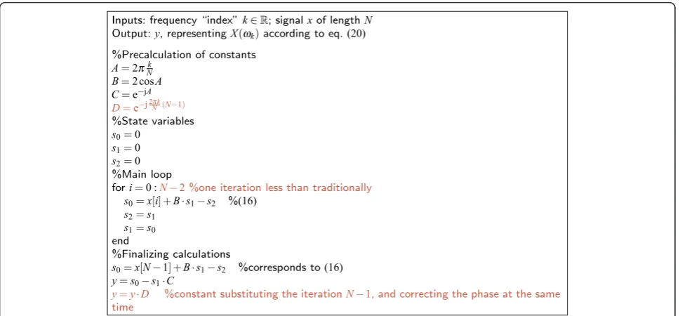
integer-valued problem, where the standard Goertzel algorithm can be utilized—so no modifications are needed. How-ever, it is at the cost of raising the computational com-plexity, which is even greater than with the generalized Goertzel algorithm (Figure 4).
Starting from (22) again, the k Î ℝ can be divided
into its integer part ⌊k⌋ Î Z and the remainder
k∈[0, 1), i.e.,k=k+k.ˆ This way, (22) can be rewrit-ten as
X(ωk) = N−1
n=0
x[n]e−j2πˆkNne−j2πk n
N. (32)
If we denote the signal created by multiplying ele-mentwise {x[n]} and {e−j2πkˆn
N}by {ˆx[n]}, the previous
relation can be written in the form of
X(ωk) = N−1
n=0 ˆ
x[n]e−j2πkNn, (33)
whose right side is a usual DFT of signal xˆ (which is complex!) and thus can be computed by the standard Goertzel algorithm.
Inputs: frequency “index”k∈R; signalxof lengthN Output:y, representingX(ωk)according to eq.(20)
%Precalculation of constants A=2πk
N B=2 cosA C=e−jA D=e−j2πk
N (N−1)
%State variables s0=0
s1=0
s2=0
%Main loop
fori=0 :N−2%one iteration less than traditionally
s0=x[i] +B·s1−s2 %(16)
s2=s1
s1=s0
end
%Finalizing calculations
s0=x[N−1] +B·s1−s2 %corresponds to(16) y=s0−s1·C
y=y·D %constant substituting the iterationN−1, and correcting the phase at the same time
Regarding the memory complexity, in case of real-time processing it is of advantage to precompute and store the signal {e−j2πkˆNn}. It is complex and therefore
requires 2Nmemory locations. Furthermore, in contrast to the traditional algorithm, we also need 2Npositions to store xˆ, which is complex (instead of Nin the tradi-tional, real case).
To compute xˆ we need 2Nreal multiplications. In the standard Goertzel algorithm (Figure 3) theNiterations of the main loop work with real numbers only (suppos-ing the input signal to be real). In the approach pre-sented above, the number of real operations is doubled.
It is therefore clear that the generalized algorithm according to Figure 4 beats the above alternative approach from both the computational and the memory viewpoints.
4 Software
Two Matlab functions are available for download at URL [10].
The function named goertzel_classic.m realizes the standard Goertzel algorithm for kÎ Z; the generalized
(and shortened) algorithm forkÎ ℝis implemented in
the function goertzel_general_shortened.m. The struc-ture of the functions corresponds to the pseudocodes in Figures 3 and 4. Indexing the vector elements, however, starts with“1”in Matlab, which differs from our theore-tical description, where it starts with“0”.
5 Conclusion
The article presented the generalization of the Goertzel algorithm. The novel approach allows us to employ also the non-integer-valued multiples of the fundamental fre-quency, making it possible to compute the Fourier transform in discrete-time (DTFT) this way. The main advantage consists in that in various applications where the Goertzel algorithm is utilized, it is no longer neces-sary to round the frequencies of desire, thus obtaining more accurate results. The article shows that this is reached at the cost of only a negligible rise in computa-tional and memory complexities. Furthermore, it has been shown that the very last iteration of the algorithm can be substituted with a multiplication which is little more effective.
Acknowledgements
This work was supported by projects of the Czech Ministry of Education, Youth and Sports MSM0021630513, the Czech Ministry of Industry and Trade FR-TI2/220, and the Czech Science Foundation 102/09/1846.
Competing interests
The authors declare that they have no competing interests.
Received: 10 May 2011 Accepted: 6 March 2012 Published: 6 March 2012
References
1. RG Lyons,Understanding Digital Signal Processing, 2nd edn. (Prentice Hall PTR, NJ, 2004)
2. P Duhamel, M Vetterli, Fast Fourier transforms: A tutorial review and a state of the art.Signal Process.19, 259 (1990). doi:10.1016/0165-1684(90)90158-U 3. H Sorensen, C Burrus, Efficient computation of the DFT with only a subset
of input or output points.IEEE Transn Signal Process.41(3), 1184 (1993). doi:10.1109/78.205723
4. SL Gay, J Hartung, GL Smith, Algorithms for Multi-Channel DTMF Detection for the WE DSP32 Family, inIEEE on Proceedings of International Conference on Acoustics, Speech, and Signal ProcessingGlasgow, 1134–1137 (1989) 5. Q.23,Technical Features of Push-Button Telephone Sets(ITU-T, Geneva, 1988) 6. P Mock, Add DTMF generation and decoding to DSP-uP designs, inDigital Signal Processing Applications with the TMS320 Family, vol. 1. (Prentice-Hall, NJ, 1987), pp. 543–557
7. G Goertzel, An algorithm for the evaluation of finite trigonometric series. Am. Math Monthly.65(1), 34 (1958). doi:10.2307/2310304
8. AV Oppenheim, RW Schafer, JR Buck,Discrete-time Signal Processing, 2nd edn. (Prentice-Hall, NJ, 1998)
9. Wikipedia contributors. inWikipedia: the Free Encyclopedia, (Wikipedia Foundation, St. Petersburg, Florida, 2010), http://en.wikipedia.org/wiki/ Goertzel_algorithm. 29. 6. 2005, 19. 1. 2010 [cit. 6. 4. 2010] 10. P Rajmic, Matlab codes for the generalized Goertzel algorithm (2012).
http://www.mathworks.com/matlabcentral/fileexchange/35103
doi:10.1186/1687-6180-2012-56
Cite this article as:Sysel and Rajmic:Goertzel algorithm generalized to non-integer multiples of fundamental frequency.EURASIP Journal on Advances in Signal Processing20122012:56.
Submit your manuscript to a
journal and benefi t from:
7Convenient online submission 7Rigorous peer review
7Immediate publication on acceptance 7Open access: articles freely available online 7High visibility within the fi eld
7Retaining the copyright to your article