R E S E A R C H
Open Access
Indoor robot localization combining feature
clustering with wireless sensor network
Xiaoming Dong
1, Benyue Su
1and Rong Jiang
2*Abstract
Indoor robot localization is an indispensable ingredient for robots to perform autonomous services because GPS (Global Position System) information is not available. Natural features are usually used to implement this task, but it is difficult to solve the problem of localization robustness. A solution is proposed combining feature clustering and wireless sensor network to improve the effectiveness of robot localization: firstly, the SIFT (scalable invariable feature transform) features are extracted with feature clustering algorithm to estimate the robot position; secondly, the wireless sensor network is constructed to localize the robot from another independent way; finally, EKF (extended Kalman filter) is utilized to fuse the two kinds of localization results. The experiments demonstrate that this proposed method is effective and robust.
Keywords:Robot, EKF, Localization, Wireless sensor network
1 Introduction
GPS is commonly used to implement robot localization, but GPS cannot be used in some conditions such as
in-door environments [1]. A common way to implement
indoor localization is to estimate robots’ pose utilizing inertial sensors; however, this method is difficult to re-solve the problem of robot’s wheel slor robot localization combining feature clusteipping, so the accumulated er-rors impact the estimating accuracy greatly [2]. In
maga-zine [3], the Non-Cooperative Feature Points are
extracted to implement the task of navigation,
which is usually based on the satellite feature points. In
magazine [4], the graph-based methods have been
car-ried out for the robot localization and navigation. In
magazine [5], the whole simulation process of robot
navigation has been implemented. The drawback of the above methods is that it is difficult to obtain the robust feature points, which are easy to be affected by light changes. Recently, wireless sensors are used in mobile robot navigation as reference nodes; the methods can be divided into two categories [6–8]: One is to implement robot localization utilizing wireless sensor networks on their own sensor nodes [9], and the other is to carry out
that on external targets [10]. This article focuses on the later that is to implement robot localization utilizing the external sensor targets. Vision features are another com-monly used in robot localization and motion estimation. According to the specific localization mechanism, exist-ing wireless sensor network localization methods can be divided into two categories [11]: A range-based method and a range-free method. The ranging-based positioning mechanism needs to measure the distance or angle in-formation between the unknown node and the anchor node, and then use trilateration, triangulation, or max-imum likelihood estimation to calculate the position of the unknown node. The non-ranging-based positioning mechanism does not require distance or angle informa-tion, or does not directly measure the informainforma-tion, and only implements node positioning based on network connectivity and other information. Localization based on ranging technology have the advantages that it can obtain higher accuracy, and the commonly used ranging technologies are RSSI (received signal strength indica-tor), TOA (time of arrival), TDOA (time difference of ar-rival) and AOA [12]. TOA (angle of arrival) is the time of arrival method. TDOA is the time difference of arrival positioning method. Both are positioning methods based on the propagation time of the waves. It is necessary to have three base stations known at the same time to as-sist in positioning. The basic principle of TOA is to get
* Correspondence:[email protected]
2School of Information, Yunnan University of Finance and Economics, Kunming 650221, China
Full list of author information is available at the end of the article
the distances from the equipment to the three base sta-tions after getting the three arrival times, and then just build the equations and solve them according to the geometry, so as to obtain the location value. TDOA does not solve the distance immediately, but calculates the time difference first, then establishes the equation group through some clever mathematics algorithm and solves, thus obtains the location value. Since the TOA calculation is completely time-dependent, the time synchronization of the system is required to be very high. Any small-time error will be amplified many times. At the same time, due to the influence of multipath, it will bring a great error, so the pure TOA is rarely used in practice. DTOA can greatly improve the accuracy of positioning because the ingeniously designed difference process cancels out a large part of the time error and multipath effect. Because DTOA has relatively low net-work requirements and high precision, it has become a research hotspot. AOA is the angle of arrival method, which is a two-base station positioning method that per-forms positioning based on the incident angle of the sig-nal. It determines the position by intersecting two straight lines, it is impossible to have multiple intersec-tions, which avoids the ambiguity of positioning. How-ever, in order to measure the incident angle of the electromagnetic wave, the receiver must be equipped with a highly directional antenna array. RSS positioning method is based on the strength of the received signal to achieve positioning. In the positioning process, the sig-nal intensity of three different reference points is mea-sured by the device, and three distance values are calculated according to the physical model. Then, a geo-metric solution method similar to TOA can be used to obtain the positioning point. Common RF chips all have RSSI measurement function, so the RSSI mechanism is easy to implement. The problem is it is susceptible to channel and noise, and it has large measurement error in long-distance positioning, which is mostly used in small-range positioning [13]. The visual information is
also commonly used to implement the robot
localization. This series of methods can be divided into monocular visual localization method and stereoscopic visual localization method [14–16]. The purpose is to use the robot vision system to sense the environment, identify the location of the road signs and obtain local map information, and continuously use the obtained local map. The main problems existing in visual localization research are it is difficult to implement fea-ture extraction and landmark recognition quickly and accurately through robot vision systems in complex en-vironments [17, 18]; the amount of image features re-quired for landmark recognition is too large, especially in a complex and large-scale environment [19, 20]. In the case of global maps, there is a problem of
information explosion. This increases the complexity and uncertainty of the localization task. Wireless sensors are flexible for robot localization, but it is difficult to achieve high accuracy only by themselves. On the other way, vision sensors are easy to be affected by many fac-tors: the degree of image distortion correction, the track-ing error of the feature points, and so on [21–23]. To improve the robustness of the robot localization, SIFT [24] and super-sphere aggregation algorithm [25] are se-lected as the vision features. The object of this paper is to develop a method integrating distinguished features of indoor environment and wireless sensor network to improve the effect of robot localization.
This paper is organized as follows: Section2described the main methods; various experiments were
imple-mented to verify the proposed method in Section 3.
Section4gives conclusions.
2 Methods
The task of robot localization is to estimate the robot’s position as well as to set up a map of the surrounding environment according to the landmarks perceived. For
the convenience of description, m represents landmark
and x represents robot position; u represents the robot
drive. In order to implement robot localization task, the distance that the robot has moved should be estimated and the position of the landmark should be calculated simultaneously. The robot updates the estimated pos-ition when the new landmark was found in the naviga-tion process. Apparently, there are some errors in the robot localization between estimation position and real position, as well as that in the landmark estimation. The target of robot localization is to reduce the estimation
errors of the robot position and surrounding
environment.
2.1 Feature clustering for robot localization
Features can be clustered to improve the robustness in robot localization. The hypersphere soft assignment [25] is used to cluster the features in our design. The principle of the hypersphere soft assignment is to con-struct a hypersphere based on each clustering center in the feature space, and the feature points are assigned to the cluster centers corresponding to the hypersphere in the space position.
The k-means algorithm is used to train K clustering
centers on a sample feature set {c1,…ci,…ck}({ciϵRk).
When the k-means algorithm converges, the feature points that are allocated to each cluster center cican be
obtained xci¼ fxi1;…xing. In which xin represents the
number of feature points assigned to the cluster center-ing ci. For each clustering center ci, the Euclidean
and the maximum distance is defined as the radius of the cluster center radiusi:
radiusi¼j¼1;2::id ci;xij
max ð1Þ
The hypersphere can be constructed in the feature space for each clustering center ci, where the radius is
radiusi. The feature points can be assigned to the
corre-sponding cluster center according to the spatial position relative to all hyperspheres.
For a feature pointxj(xjϵRd), aKdimensional
attribu-tion vector attribj= {attribj1,…, attribjk} is defined, where
attibjiindicates whether the feature point xjis allocated
to the clustering center: attribji= 1 represents that xj is
allocated to ci, attribij= 0 represents that it is not
allo-cated to ci. The characteristic this soft allocation
mech-anism of the hypersphere is represented as follows:
attribji¼ 0 when d xj;ci
Only when the Euclidean distance between the feature pointxjand the cluster centerciis less than or equal to
the corresponding radius of the super sphere, xj would
be allocated toci. The value of component attribjiin the
corresponding vector attribjis set to 1.
a, b,…,Iare assumed as the clustering centers, and x1,
x2,x3, andx4are the four feature points to be allocated. The policy of soft assignment can be described as fol-lows: firstly, the hypersphere needs to be constructed for each clustering center, where the clustering center is set as the center of the corresponding hypersphere. The clustering centers are assumed as b,c,d, andewith the corresponding circles; secondly,x1, x2,x3, andx4will be assigned to a cluster center according to whether they are located within the corresponding circle. For example,
x1 is only located within the circle corresponding to b, so x1is only assigned to b; feature points as x3and x4 are located within the circles corresponding to b and c, so the x3 and x4 are both allocated to b and c; x2 is
located within the circles corresponding to c, d, and
e, it will be allocated to the c, d, and e as three clus-ter cenclus-ters.
Given a feature pointxj, a K dimension weight vector
wj= {wj1,…wjk} is defined, where the vector component
wjirepresents the weight of the clustering centerci
rela-tive to xj. It is assumed that the Euclidean distance
be-tween the feature points and the nearest neighbor clustering center is subject to the Gaussian mixed distri-bution. Therefore, the weight can be calculated accord-ing to the formula.
dij is defined as the Euclidean distance, which is set
from feature point xj to clustering center ci; σ is the
standard deviation, which is assumed to be Gaussian mixture distribution. The optimal value can be
deter-mined through experiments. The weight vectors wj
needs to be L1 normalized, so that the weights of the
cluster centers are calculated as follows.
wji¼
VLAD is the abbreviation of “vector of locally aggre-gated descriptors,” which is an image descriptor aggre-gating the local features of the SIFT in the feature space. VLAD is proposed on the basis of the method of the BOF (bag of features) image descriptor, combined with the idea of the Fisher kernel. Similar to the BOF image descriptor, VLAD takes the K-means clustering algo-rithm as a training set to get k clustering centers. Each cluster center is called a visual word, and the set of K
visual words is called a codebook C= {c1,…ci,…
ck}({ciϵRk).
The soft assignment method can be combined with VLAD when it is used to generate the image descriptor SSA-VLAD (Spherical Soft Assignment vector of locally aggregated descriptors). The way is similar to VLAD: a sample set is trained to obtain the codebook, which in-cludes K cluster centers utilizing the K-means clustering algorithm. Differing from VLAD, the corresponding ra-dius needs to be calculated for each visual word (the clustering center) in the training ofC.
For an image, after extracting the local features of the SIFT X= {x1,…xi,…xk}, the specific steps for its
SSA-VLAD generation are as follows:
Step1: Using the hypersphere soft allocation method, each SIFT featurexjis assigned to the
adjacent visual words to obtain the attribution vector attribj.
Step2: Computing the weight vectorwjof the
SIFT featurexjrelative to the nearest neighbor
visual word.
Step3: The weighted vector residuals, which is the SIFT featurexjrelative to the nearest neighbor
Step4: For each visual wordCi, allocate it for aggregation
to the corresponding weighted residuals vector among all the featuresxjbelonging to the visual word.
Step5: The K aggregation vectorviis connected in
series to form an SSA-VLAD vector {v1,…vi,…vk},
wheredis the vector dimension of the SIFT feature.
The vector dimension of SSA-VLAD is the same as VLAD, which isk×d.
2.2 Robot localization based on wireless sensor network
The centroid localization algorithm is chosen as the auxil-iary location method, which has the most important ad-vantages: the little time consumption and the fast location speed. The essential of centroid algorithm is that the robot can use the geometric centroid of anchor nodes in the range of communication as its location estimation. The concrete process can be described as follows:
Anchor nodes broadcast a beacon signal to neighbor nodes’set intervals, which contains ID and location infor-mation of anchor nodes themselves. When the number of beacon signals that the robot received from an anchor node exceeds a predetermined threshold in a fixed period, the robot is considered to be connected to the anchor node and its position can be determined as the polygon centroid composed of all connected anchor nodes. The geometric center of polygon is called centroid; the coordi-nates of the centroid are the average value of polygonal vertex coordinates. Assumed that the vertex coordinates of polygonal are (x1, y1), (x2, y2)…(xn,yn), respectively, the
centroid coordinates can be calculated as:
Xt;Yt
The robot position can be obtained according to the centroid coordinates, and the error of localizationWtis
assumed as Gaussian distribution.
2.3 Robot localization combing feature clustering and WSN with EKF
2.3.1 EKF process in robot localization
Kalman filter is usually used as state estimation or par-ameter estimation for a system, which updates the
math-ematical expectation and covariance of Gaussian
probability distribution under Bayesian theory frame-work. By minimizing the square of the deviation between the real state and the estimated state of the system, Kal-man filter provides an effective estimation method for the system’s present and future state without the exact model of the system.
There is a requirement in the classic Kalman filter that a control system is linear, but most practical control sys-tems are nonlinear. Therefore, the extended Kalman fil-ter (EKF) is used in our design, where the nonlinear control process and the measurement model are linear-ized to make the traditional Kalman filter be appropriate for the nonlinear systems.
But EKF has two obvious shortcomings: first, derivation of the Jacobian matrix and linear estimation of nonlinear equations may be very complex, contributing to the diffi-culties in real applications; secondly, when the filter time step is not small enough, the linearization for nonlinear equations will lead to system instability.
The EKF extends the motion model and the observa-tion model of the system to the nonlinear condiobserva-tion, and its motion model can be expressed as:
xt¼ f xð t−1;ut−1;wt−1Þ ð8Þ
where tdenotes the discrete time, xdenotes robot
pos-ition, andudenotes the distance that robot has run from the last time step to the current time step. Additionally,
wt−1denotes the noise distribution in timet-1. The ob-servation model can be described as Eq.9, wherevt
de-notes the observation noise and zt denotes the
observation results:
zt ¼h xð t;vtÞ ð9Þ
The state prediction and the observation prediction are defined as follows respectively, where^x−t denotes the prediction value of robot position:
^x−t ¼ f ^xt−−1;ut−1;0
The EKF filtering algorithm is linearized through Tay-lor expansion to linearize the nonlinear motion model and observation model, and then, the update process can be obtained according to the similar way as Kalman filtering.
The time update equation in EKF can be represented as Eq.12, whereP^−t denotes the variance:
^
P−t ¼AtPt−1ATt þWtPQt−1WTt ð12Þ
Kt ¼P−tHTt HtP−tHTt þVtRtVTt
Considering that the position of the measured land-mark is not accurate absolutely. The appropriate motion model and observation model should be set up to analyze the robot localization error. In our designed ex-periment, the wheel robots are selected and its driven model can be set up as follows.
2.3.2 Robot model
Because the robot selected in this paper is a wheel robot, the model can be described as follows:SL is assumed as
the distance that the left wheel moves, andSRis the
dis-tance that the right wheel moves. Δθ is the wheel axis
rotation angle, and θ represents the intersection angle. Then, the change of robot poses between the current one and the last one can be estimated, whereXi(xi,yi,θi)
is the current robot pose, and Xi(xi−1,yi−1,θi−1) repre-sents the last one. So, the relation between the robot ro-tation angle and the distance that the robot moves can be calculated according to Eq. 14. The arc length is the distance that the robot center has moved, which can be represented as Eq.15, andDcan be calculated based on Eq.16:
The current pose update can be described as the Eq. 17. Considering the effect of noise, the formula of the
robot pose can be changed to Eq.18. Among whichWi
−1is the Gaussian noise that is assumed ordinarily:
Xi¼Xi−1þðΔx;Δy;ΔθÞ ð17Þ
Xi¼ F Xð i−1;SLi−1;SRi−1Þ þWi−1 ð18Þ
Covariance could be described as a diagonal matrix, and the diagonal entries are shown in Eq.19:
Q11¼KxjS cosð Þθ j
Among which Kx and Ky are the robot drift
coeffi-cients, which are along the x-axis and the y-axis simi-larly, KSθ and Kθθ are the robot drift coefficients of
angles. The values of the coefficients can represent the error in this model.
2.3.3 Observation model
There are some errors in the estimation of robot move-ment contributing to the robot movemove-ment model, as well as the observation error. The observation model is an-other important aspect in robot localization. The
obser-vation position of the ith landmark can be deduced as
Eq.20:
In Eq. 20, the observation noise can be ordinarily as-sumed as Gaussian noise, among which the average is assumed to zero, and covariance matrix is assumed as diagonal matrix.
3 Experiment results and analysis
The Institute of Automation of Chinese Academy of Sci-ences has independently developed a versatile autono-mous mobile robot platform called AIM based on its existing technology. The various theories and algorithms described in this paper are tested on the platform. The vision sensor is placed on the top of the mobile robot.
The feature clustering algorithms of VLAD [26] and
RNN-VLAD [27] are selected for the better comparison.
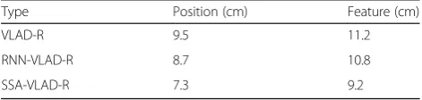
The VLAD method is like BOF, which considers only the nearest cluster center of the feature points that saves each feature point to its closest cluster center distance. Like the Fisher vector, VLAD considers the value of each dimension of the feature points and has a more detailed description of the local information of the image. The most advantage in VLAD is that there is no loss of infor-mation on the VLAD features. The standard deviations of estimation errors for different algorithms are summa-rized in Table1. It is worth noting that each value in this table averages the whole results. In RNN-VLAD, a set of descriptors were extracted from each observed image se-quence, and the deformations of each image sequence were analyzed. Finally, each descriptor was assigned to the nearest visual center. The standard deviations were calculated to compare the effectiveness of motion esti-mation based on the different kinds of methods. For the
Table 1Standard deviation of different aggregation algorithm
Type Position (cm) Feature (cm)
VLAD-R 9.5 11.2
RNN-VLAD-R 8.7 10.8
convenience of description, the method of robot localization based on VLAD is represented as VLAD-R, and RNN-VLAD-R represents the localization method based on RNN-VLAD. Similarly, SSA-VLAD-R repre-sents the localization method based on SSA-VLAD. Ac-cording to comparison results, the standard deviations of SSA-VLAD are smaller than RNN-VLAD, while the standard deviations of RNN-VLAD are smaller than ori-ginal VLAD.
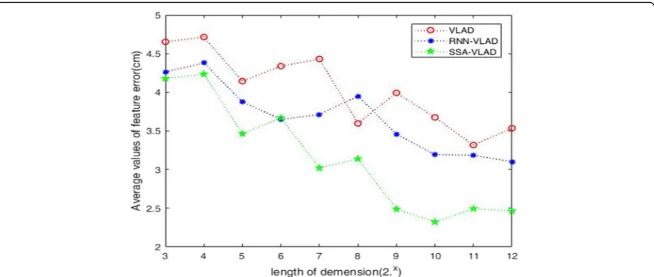
Different dimension lengths have important impacts on the estimation of feature errors and position errors for different algorithms. For the better comparison, we
analyze the results of dimension lengths from different angles. As shown in Figs.1,2,3, and4. The relation be-tween the location accuracy and dimension lengths was analyzed.
The average mean square values of feature error for dif-ferent algorithms are shown in Fig.1. The average feature error is smaller as dimension length increases. Among the three algorithms, the worst algorithm is the localization based on original VLAD, which has the largest feature es-timation error. The best algorithm is the proposed method based on SSA-VLAD, which has the smallest fea-ture estimation error for the same dimension length. Fig. 1The average values of feature error with different lengths of dimension. Legend: Thex-axis denotes the dimension length, and they-axis denotes the average values of feature error (cm)
The average position error values for different algo-rithms and different dimension length are shown in Fig. 2. It is shown that the average position errors of the three algorithms become smaller as dimension length increases. The worst algorithm is the method based on original VLAD, which has the largest aver-age position error. The best algorithm is still the pro-posed method based on SSA-VLAD, which has the smallest position estimation error for the same di-mension length.
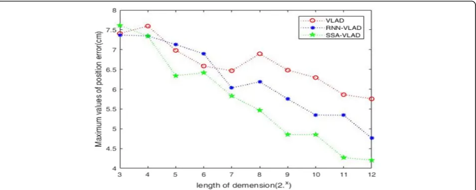
Figure 3 shows the impact of different dimension
lengths in maximum mean square estimation of feature,
and Fig. 4 shows that of position. In these conditions,
the method based on SSA-VLAD has the best results for each same dimension length, and the method based on RNN-VLAD is better than the method based on ori-ginal VLAD.
4 Conclusions
In this paper, the robot localization based on feature
clustering algorithm was proposed, and robot
localization utilizing wireless sensor network is inte-grated to improve the robustness. The performance of proposed algorithm was verified by reduced feature er-rors and robot position erer-rors. The various experiment results show that the localization problem can be solved Fig. 3The maximum values of feature error with different lengths of dimension legend: Thex-axis denotes the dimension length, and they-axis denotes the maximum values of feature error (cm)
better, and the efficiency of localization was improved. Moreover, the proposed algorithm can still achieve satis-fied estimation accuracy even when either feature cluster-ing algorithm or wireless sensor network localization algorithm fails. In future work, the robustness of feature clustering algorithm will be analyzed further and different filter algorithms would be implemented to improve the localization efficacy in distinguished indoor environments.
Acknowledgements
The paper was supported by the National Natural Science Foundation of China (nos. 61763048, 61263022, and 61303234), National Social Science Foundation of China (no. 12XTQ012), Science and Technology Foundation of Yunnan Province (no. 2017FB095, 201801PF00021), and the 18th Yunnan Young and Middle-aged Academic and Technical Leaders Reserve Personnel Training Pro-gram
(no. 2015HB038). It is also supported by the Foundation of University Research and Innovation Platform Team for Intelligent Perception and Computing of Anhui Province, key research project of natural science of Anhui Provincial Education Department (no. KJ2017A354). The authors would like to thank the anonymous reviewers and the editors for their suggestions.
Authors’contributions
RJ and XD designed the experiments and wrote the paper. RJ and XD performed the experiments. BS analyzed the data. All authors have read and approved the final manuscript.
Author’s information
Xiaoming Dong received his M.S. and Ph.D. degree from Automation of Institution, Chinese Academy of Sciences in 2010. He is currently an associate professor at the school of computer and information, Anqing Normal University and the key laboratory of intelligent perception and computing of Anhui Province. His research interests lie in robot navigation, wireless sensor networks, pattern recognition, image processing, and Internet of Things (E-mail: [email protected]).
Benyue Su received the Ph. D. degree from Hefei University of Technology in 2007. He is currently a professor at the school of computer and information, Anqing Normal University and the key laboratory of intelligent perception and computing of Anhui Province. His research interests lie in machine learning, pattern recognition, image processing, and computer graphics (E-mail: [email protected]).
Rong Jiang* received his Ph.D. degree in system analysis and integration from the school of software at Yunnan University. He is currently a professor and Ph. D. supervisor at the school of information, Yunnan University of Finance and Economics, China. He has published more than 30 papers and ten books and has gotten more than 40 prizes in recent years. His main research interests include cloud computing, big data, software engineering, information management, and pattern recognition (E-mail:
Competing interests
The authors declare that they have no competing interests.
Author details
1The University Key Laboratory of Intelligent Perception and Computing of Anhui Province, Anqing Normal University, Anhui 246133, China.2School of Information, Yunnan University of Finance and Economics, Kunming 650221, China.
Received: 7 May 2018 Accepted: 11 June 2018
References
1. J Fuentespacheco, J Ruizascencio, JM Rendonmancha, et al., Visual simultaneous localization and mapping: a survey[J]. Artif. Intell. Rev.43(1), 55–81 (2015).
2. A Kim, RM Eustice, Active visual SLAM for robotic area coverage: theory and experiment[J]. Int. J. Robot. Res.34(4), 457–475 (2015).
3. S Hara, D Anzai, inIEEE Vehicular Technology Conference. Experimental Performance Comparison of RSSI- and TDOA-Based Location Estimation Methods, vol. 2008 (Vtc Spring, 2008) pp. 2651–2655.
4. M Ning, S Zhang, S Wang, A non-cooperative satellite feature point selection method for vision-based navigation system. Sensors18, 854 (2018). 5. K Eckenhoff, L Paull, G Huang, inIEEE International Conference on Intelligent
Robots and Systems(IROS), Decoupled, consistent node removal and edge sparsification for graph-based SLAM[C]. Vol. 2016. pp. 3275–3282. 6. T Bailey, HF Durrantwhyte, Simultaneous localization and mapping (SLAM):
part II[J]. IEEE Rob. Autom. Mag.13(3), 108–117 (2006).
7. A Awad, T Frunzke, F Dressler,in Proceedings of the 10th Euromicro Conference on Digital System Design Architectures, Methods and Tools
Adaptive Distance Estimation and Localization in WSN Using RSSI Measures. (DSD, Lubeck, 2007) pp. 471–478.
8. Y Kong, Y Kwon, G Park, Robust localization over obstructed interferences for inbuilding wireless applications. IEEE Transactions on Consumer Electronics,55(1), 105-111 (2009).
9. HS Ahn, W Yu. Environmental-Adaptive RSSI-Based Indoor Localization[J]. IEEE Transact. Autom. Sci. Eng.6(4):626–633 (2009)
10. AS Paul, EA Wan, RSSI-Based Indoor Localization and Tracking Using Sigma-Point Kalman Smoothers[J]. IEEE J. Sel. Top. Sig. Process.3(5):860–873 (2009). 11. H Ren, QH Meng, Power Adaptive Localization Algorithm for Wireless
Sensor Networks Using Particle Filter[J]. IEEE Transact. Veh. Technol.58(5): 2498–2508 (2009).
12. YY Cheng, YY Lin, A new received signal strength based location estimation scheme for wireless sensor network[J]. IEEE Transact.Consum. Electron.55(3): 1295–1299 (2009).
13. K Kleisouris, Y Chen, J Yang, et al., Empirical Evaluation of Wireless Localization when Using Multiple Antennas[J]. IEEE Transact Parallel Distributed Syst.21(11):1595–1610 (2010).
14. C Jinwoo et al., inSICE-ICASE, 2006. International Joint Conference. A practical solution to SLAM and navigation in home environment (2006).
15. V Indelman, No correlations involved: decision making under uncertainty in a conservative sparse information space[J]. IEEE Robot. Autom. Lett.1(1), 407–414 (2017).
16. Jonathan, H Zhang, inThe Fourth Canadian Conference on Computer and Robot Vision. Quantitative evaluation of feature extractors for visual SLAM (2007). 17. J Wu, J Li, W Chen, Practical adaptive fuzzy tracking control for a class of
perturbed nonlinear systems with backlash nonlinearity. Inf. Sci.420, 517– 531 (2017).
18. L Carlone, R Tron, K Daniilidis, et al., inInternational Conference on Robotics and Automation. Initialization techniques for 3D SLAM: a survey on rotation estimation and its use in pose graph optimization[C] (2015).
19. H Carrillo, P Dames, V Kumar, et al., inInternational Conference on Robotics and Automation. Autonomous robotic exploration using occupancy grid maps and graph SLAM based on Shannon and Rényi entropy[C] (2015). 20. G Silveira, E Malis, P Rives, inIEEE International Conference on Robotics and
Automation. An efficient direct method for improving visual SLAM (2007). 21. W Jian, Z-G Wu*, J Li, G Wang, H Zhao*, W Chen, Practical adaptive fuzzy control of nonlinear pure-feedback systems with quantized nonlinearity input. IEEE Trans. Syst. Man Cybern. (2018).https://doi.org/10.1109/TSMC. 2018.2800783.
22. A Sunghwan et al., inRobotics and Automation, 2007 IEEE International Conference on. SLAM with visual plane: extracting vertical plane by fusing stereo vision and ultrasonic sensor for indoor environment (2007). 23. A Sunghwan et al., inIEEE/RSJ International Conference on Intelligent Robots
and Systems. Data association using visual object recognition for EKF-SLAM in home environment (2006).
24. DG Lowe, Distinctive image features from scale-invariant keypoints[J]. Int. J. Comput. Vis.60(2), 91–110 (2004).
25. AI Liefu, YU Junqing, WU Zebing, Y He, T Guan, Optimized residual vector quantization for efficient approximate nearest neighbor search. Multimedia Systems23(2), 169–181 (2017).
26. J Herve, D Matthijs, S Cordelia, et al., inIEEE Conference on Computer Vision and Pattern Recognition (CVPR). Aggregating local descriptors into a compact image representation (2010), pp. 3304–3311.