VRP-GMRES(m) Iteration Algorithm for Fast
Multipole Boundary Element Method
Chunxiao Yu, Cuihuan Ren * and Xueting Bai
College of Science, Yanshan University, Qinhuangdao 066004, China; [email protected] * Correspondence: [email protected]; Tel.: +1-871-351-0209
Abstract: To solve large scale linear equations involved in the Fast Multipole Boundary Element Method (FM-BEM) efficiently, an iterative method named the generalized minimal residual method (GMRES)(m)algorithm with Variable Restart Parameter (VRP-GMRES(m) algorithm) is proposed. By properly changing a variable restart parameter for the GMRES(m) algorithm, the iteration stagnation problem resulting from improper selection of the parameter is resolved efficiently. Based on the framework of the VRP-GMRES(m) algorithm and the relevant properties of generalized inverse matrix, the projection of the error vectorrm+1onrmis deduced. The result proves that the proposed algorithm is not only rapidly convergent but also highly accurate. Numerical experiments further show that the new algorithm can significantly improve the computational efficiency and accuracy. Its superiorities will be much more remarkable when it is used to solve larger scale problems. Therefore, it has extensive prospects in the FM-BEM field and other scientific and engineering computing.
Keywords: FM-BEM; variable restart parameter; GMRES(m); error vector projection; convergence
1. Introduction
Mathematical models of partial differential equations are usually established for many problems in scientific and engineering fields. After discretization, the equations can be concluded as the solution of a large scale linear system of equations, which can be expressed as
Ax=b,A∈Rn×n, x, b∈Rn, (1)
For the GMRES(m) algorithm, the selected parametermis fixed during the whole iterative process; therefore, the selection ofmis one of the key factors for the algorithm implementation. Research shows that a small value ofmmay result in slow convergence or no convergence, while a large value ofmwill cause too much of a memory requirement. Therefore, the appropriate selection of parametermis a trouble for many scholars.Recently, some researchers have tried to overcome these difficulties by changing the restart parametermin the GMRES(m) algorithm. Baker tried to improve the convergence by selecting an arbitrary parameterm. In addition, he tried it by determining the parametermaccording to the continuous two times of residual norms ratio[26,27].However, the effect was not so good. Peairs determined the value of mby a reinforcement learning method, which indicated that proper changing ofmcould improve the computational efficiency.However, it was only a kind of machine learning method. Thus, it had certain limitations [28].
In this paper, the GMRES(m) algorithm combined with the FM-BEM is studied, and a new kind of GMRES(m) algorithm with Variable Restart Parameter (VRP-GMRES(m) algorithm) is presented. By appropriately changing a variable restart parameter, the new algorithm can effectively avoid many disadvantages caused by improper selection of parametermin the GMRES(m) algorithm. At the same time, the computational efficiency and accuracy will be greatly improved.
2. Fundamental Theory for the GMRES(m) Algorithm 2.1. Galerkin Principle
Given an arbitrary initial valuex0∈Rn. Letx=x0+z, and then Equation (1)is equivalent to
Az=r0, (2)
wherer0=b−Ax0indicates the initial residual vector. Suppose thatKmandLmare twom-dimensional Krylov subspaces inRn, and they are formed by
Km=spannr0,Ar0,· · ·,Am−1r0
o
,
Lm=spannAr0,A2r0,· · ·,Amr0
o
=AKm.
Letv1, v2, · · · ,vmandw1, w2, · · · ,wmbe the bases ofKmandLm, respectively;Vm={vi}mi=1 andWm={wi}mi=1. For the solution of Equation (2), the Galerkin principle can be described as follows: give a fixed m > 0, and find an approximate solution zm ∈ Km, so that(r0−Azm)⊥Lm, namely,
(r0−AVmym)⊥Lmor(r0−AVmym, wi) =0 ,ym∈Rm.
2.2. Arnoldi Process
The Arnoldi process can be described as follows:
1. For the givenm>0 andx0∈ Rn, computev1=r0kr0k,r0=b−Ax0. 2. Whenk = 1, 2,· · ·, m, computevk+1 = Avk−
k ∑ i=1
hi,kvi,hi,k = (Avk,vi)andhk+1,k = kvk+1k, respectively. It is obvious thatvk+1⊥vi (i=1, 2,· · ·,k).
3. Ifhk+1,k =0, thenvk+1=0 and stop. Otherwise, letvk+1=vk+1
hk+1,k. The Arnoldi process has the following important property:
Theorem 1. In the Arnoldi process, let Vm+1= (Vm|vm+1)and Hm=
"
Hm hm+1,meTm
#
, and then we have the following relationship [29]:
AVm=VmHm+hm+1,mvm+1eTm, AVm=Vm+1Hm, VTm+1Vm+1=I,
where Hm = (hij)mis an upper Hessenberg matrix, eTm = (0, 0, · · ·, 1)∈ Rm, and I is an m+1order identity matrix .
2.3. GMRES(m) Algorithm
Theorem 2. Suppose that A ∈ Rn×n and Lm = AKm, x = x0+z = x0+Vmy. Then, the approximate
solution zmobtained from the Galerkin principle makes the residualkr0−Azkbe at a minimum in the Krylov
subspaceKm, and the residual satisfies [30]
krk=kb−Axk=kr0−Azk=
βe1−Hmy
, (4)
whereβ=kr0k, e1= (1, 0, · · ·, 0)T∈Rm+1. Theorem 2indicates that min
zm∈Km
kr0−Azmk = min
y∈Rm
βe1−Hmy
. The basic thought of the
GMRES(m) algorithm is to give a fixed restart parametermand computezmby an iterative procedure so thatkrmk=kr0−Azmk<ε, ∀ε>0 .
The GMRES(m) algorithm includes the following steps:
1. Give a fixed integerm <<nand an initial valuex(0) ∈ Rn, computer(0) =b−Ax(0), and let r0=r(0).
2. Obtain{vi}mi=1andHmthrough the Arnoldi process . 3. Solve the least squares problem
min y∈Rm
βe1−Hmy
to obtainym, wheree1= (1, 0,· · ·, 0)T∈Rm+1. Then, computezm=Vmym.
4. Form an iterative processx(k+1)=x(k)+zm orr(k+1)=r(k)−Azm, k=0, 1, 2,· · ·. 5. If
r
(k+1)
<ε, thenx∗ ≈ x
(k+1)and stop .Otherwise, letr
0=r(k+1), and go to 2.
For the GMRES(m) algorithm, arbitrary selection of parametermcannot guarantee convergence. In fact, appropriate change ofmcan effectively improve the convergence and avoid the phenomenon of slow convergence or even no convergence.
3. VRP-GMRES(m) Algorithm
3.1. VRP-GMRES(m) Algorithm
The basic thought of the VRP-GMRES(m) algorithm is to appropriately change the restart parameter m and carry out iterative procedures so that the residual vector satisfies krmk = kr0−Azmk<ε, ∀ε>0. It includes the following main steps :
1. Give an integerm << n and an initial valuex(0) ∈ Rn, compute r(0) = b−Ax(0), and let r0=r(0).
2. Carry out the Arnoldi process and obtain{vi}mi=1andHm. 3. Solve the least squares problem
min y∈Rm
βe1−Hmy
(5)
and getym. Then, computezm=Vmym.
4. Form an iterative process byx(k+1)=x(k)+ zm, k=0, 1, 2,· · · Computer(k+1)=b−Ax(k+1). 5. If
r
(k+1)
< ε. Then,x∗ ≈ x
(k+1)and stop. If r
(k+1)
≥ ε, then letr0 = r
For the VRP-GMRES(m) algorithm, slow convergence or no convergence rarely occurs. However, the memory requirement will grow with the increase of parameterm, which can be cleverly avoided. Whenmincreases to some extent and the residual norm reduces to a proper value, the parameterm can be fixed and the GMRES(m) algorithm will be carried out .
3.2. Convergence Analysis
Definition 1. Suppose thatA∈Cm×n,X∈Cm×n, at the same time if
AXA=A, XAX =X, (AX)H =AX, (XA)H =XA,
thenXis the pseudo inverse matrix ofA, denotedA+, namelyX=A+[31].
Theorem 3. Suppose that A ∈ Cm×n, and A = BC is the maximum rank decomposition of A, then X = CH(CCH)−1(BHB)−1BHis the pseudo inverse matrix of A.
Proof of Theorem 3.
AXA=BCCH(CCH)−1(BHB)−1BHBC=BC=A, XAX=CH(CCH)−1(BHB)−1BHBCCH(CCH)−1(BHB)−1BH
=CH(CCH)−1(BHB)−1BH =X.
Hereto, the first two Moore Penrose equations are established. The following is to verify the other two Moore Penrose equations:
(AX)H = [BCCH(CCH)−1(BHB)−1BH]H = [B(BHB)−1BH]H =B(BHB)−1BH= AX,
(XA)H = [CH(CCH)−1(BHB)−1BHBC]H= [CH(CCH)−1C]H =CH(CCH)−1C=XA,
From Definition1, the matrixXis a pseudo inverse matrix ofA.
Corollary 1. Suppose that A∈Cm×nis a matrix with full column rank. Then, we have
A+=AHA−1AH. (6)
Theorem 4. Suppose that rmand rm+1are the error vector of the m cycle and m+1, respectively. Then, the
following relationship is established:
coshrm,rm+1i=
krm+1k2 krmk2 .
Proof of Theorem 4. For the VRP-GMRES(m) algorithm, whenm=m+1 , the subspaceKmbecomes Km+1=span{rm, Arm, · · ·, Amrm}.
From the Arnoldi process, {vi}im=+11 and ¯Hm+1 are obtained, where v1 = rmβ, β = krmk2, coshrm,rm+1i=coshv1,rm+1i= v
From Equation (5), the least squares solutionym+1=H¯+m+1(βe1), e1 ∈Rm+2is obtained, where ¯
Hm++1is a real matrix with full column rank. According to Equation (6),we have
¯
Hm++1=H¯mT+1Hm¯ +1
−1
¯ HmT+1. Then,
ym+1=
¯
HmT+1Hm¯ +1
−1
¯
HmT+1(βe1), e1 ∈Rm+2. (7) On the other hand, we have
rm+1=b−Axm+1=b−A(xm+Vm+1ym+1) =rm−AVm+1ym+1. Accrording to Equation (3), we haveAVm+1=Vm+2Hm¯ +1. Then, we have
rm+1=rm−Vm+2Hm¯ +1ym+1=βv1−Vm+2Hm¯ +1ym+1. Thus,
krm+1k22= (βv1−Vm+2Hm¯ +1ym+1)T(βv1−Vm+2Hm¯ +1ym+1)
=β2−βvT1Vm+2H¯m+1ym+1−βym+1TH¯mT+1Vm+2Tv1
+yTm+1H¯Tm+1VmT+2Vm+2Hm¯ +1ym+1
=β2−βhTym+1−(βym+1TH¯mT+1Vm+2Tv1 −βyTm+1H¯mT+1VmT+2Vm+2H¯m+1 H¯Tm+1H¯m+1
−1 ¯
HT
m+1e1)
=β2−βhTym+1=β(β−hTym+1). At the same time, because
vT1rm+1=vT1(βv1−Vm+2Hm¯ +1ym+1) =β−hTym+1 (hTindicates a vector formed by the first line elements in ¯Hm+1), follows
cos hrm,rm+1i=
β−hTym+1
p
β(β−hTym+1)
= krm+1k2
krmk2 . (8)
Theorem 5. For the VRP-GMRES(m) algorithm, let E=krmk2, ¯E=krm+1k2, and thereforeE¯ <E.
Proof of Theorem 5. In Equation (8), coshrm,rm+1i ≤1, namely, krm+1k2
BecausehTym+16=0, it follows ¯
E=krm+1k2<krmk2=E. (9)
4. Numerical Experiments
In this section, three different types of numerical experiments are given to illustrate the validity and feasibility of the VRP-GMRES(m) algorithm. In Example 1 and Example 2,take x(0)= (0, 0,· · ·, 0)T∈R(n−1)2 as the initial value and
ε=1×10⁻⁸as the convergence criterion.
Example 1. Consider the following one-dimensional Wave equation:
utt=4uxx, 0<x<1, 0<t<0.5, u(0,t) =u(1,t) =0, 0≤t≤0.5,
u(x, 0) = f(x) =sin(πx) +sin(2πx), 0≤x≤1, ut(x, 0) =g(x) =0, 0≤x≤1.
(10)
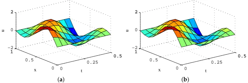
As is shown in Figure1a, the exact solution isu(x,t) =sin(πx)cos(2πt) +sin(2πx)cos(4πt), whereu(x,t)indicates the amplitude. For the problem expressed by Equation (10),nequall divisions along thex-direction andt-direction can be obtained by the central difference method.
Ax=b, A∈ R(n−1)2×(n−1)2, x,b∈R(n−1)2. (11) Equation (11) is solved by the VRP-GMRES(m) algorithm, and the numerical results are shown in Figure1b. From Figure1, the numerical solution is consistent with the exact solution.
0
0.25
0.5 0.5
0 0.5 1 1 −2 0 2 2
t x
u
(a)
0
0.25
0.5 0.5
0 0.5 1 1 −2 0 2 2
t x
u
(b)
Figure 1.Amplitude distribution(n=10,m=7). (a) exact solution; and (b) numerical solution.
0.1 0.4
0.7 0.90.9
0.05 0.25 0.45 0.45 0 0.5 1 1.5 2 2.5 2.5 x t
error for GMRES(m)
(a)
0.1 0.4
0.7 0.90.9
0.05 0.25 0.45 0.45 0 0.5 1 1.5 1.5 x t
error for VRP−GMRES(m)
(b)
Figure 2. Absolute errors after two iterations. (a) generalized minimal residual method (GMRES)(m) algorithm; (b) Variable Restart Parameter(VRP)-GMRES(m) algorithm.
0.1 0.4
0.7 0.90.9
0.05 0.25 0.45 0.45 0 0.5 1 1.5 2 2.5 x t
error for GMRES(m)
(a)
0.1 0.4
0.7 0.90.9
0.05 0.25 0.45 0.45 0 3 6 9 9
x 10−15
x t
error for VRP−GMRES(m)
(b)
Figure 3.Absolute errors after three iterations. (a) GMRES(m) algorithm; (b) VRP-GMRES(m) algorithm.
From Figures2and3, for the same number of iterations, we can see that the absolute errors generated from the VRP-GMRES(m) algorithm are much smaller than those from the GMRES(m) algorithm. With the increase in the number of iterations, the errors from the VRP-GMRES(m) algorithm reduces much faster. It shows that the new algorithm not only has higher computational accuracy, but can also speedily converge.
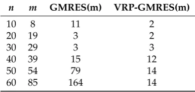
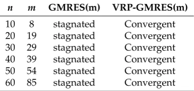
The parameters n and m are taken as different values and the calculation results from the two algorithms are compared. Tables1–4show the iteration times, computation time, computational accuracy and convergence, respectively. From Tables1–3, we can see that the new algorithm is fast convergent, stable, highly accurate and effective. From Tables1–4, the selection of parametermis very important for the GMRES(m) algorithm, and the improper parametermwill result in an algorithm failure. However, it has no effect on the VRP-GMRES(m) algorithm because the variable restart parametermcan partly reduce the sensitivity ofm.
Table 1.Comparison of iteration times for the two algorithms.
n m GMRES(m) VRP-GMRES(m)
10 8 11 2
20 19 3 2
30 29 3 3
40 39 15 12
50 54 79 14
Table 2.Comparison of computation times for the two algorithms.
n m GMRES(m) VRP-GMRES(m)
10 8 0.029415 s 0.018254 s
20 19 0.028982 s 0.013442 s
30 29 0.092144 s 0.086172 s
40 39 1.381825 s 0.847108 s
50 54 23.539635 s 4.683026 s 60 85 157.340531 s 14.662790 s
Table 3.Comparison of computational accuracy for the two algorithms.
n m GMRES(m) VRP-GMRES(m)
10 8 2.1069×10⁻⁹ 2.9235×10⁻¹⁴ 20 19 1.1751×10⁻¹⁵ 1.1984×10⁻¹⁵ 30 29 2.0093×10⁻¹² 5.4751×10⁻¹⁴ 40 39 2.4647×10⁻⁹ 2.1327e×10−10 50 54 3.3092×10⁻¹¹ 2.0783×10⁻¹¹ 60 85 2.0593×10⁻⁹ 6.5913×10⁻¹³
Table 4.Comparison of convergence for the two algorithms.
n m GMRES(m) VRP-GMRES(m)
10 8 stagnated Convergent
20 19 stagnated Convergent
30 29 stagnated Convergent
40 39 stagnated Convergent
50 54 stagnated Convergent
60 85 stagnated Convergent
In fact, the condition number of coefficient matrix A keeps growing with the increase of n. Whenn= 60, it reaches 2.1098×10³, which makes Equation (11) become severely ill-conditioned. From Table1, under the same accuracy, the number of iterations for the GMRES(m) algorithm is 11.7 times larger than that for the VRP-GMRES(m) algorithm, and the computation time is 10.7 times larger. With the increase of computing scale, the VRP-GMRES(m) algorithm will be much more effective, and its engineering application prospect is much wider.
Example 2. Consider the following two-dimensional Poisson equation:
(
uxx+uyy=2 3x+x2+y2
, (x,y)∈Ω, u(x,y) =x2 x+y2
+2, (x,y)∈∂Ω, (12) whereΩ={(x,y)|0≤x≤1, 0≤y≤1}.
The exact solution isu(x,y) =x2 x+y2
+2, which indicates a temperature distribution function. The temperature distribution is shown in Figure4a. For the problem expressed by Equation (12),nequal divisions along the x-direction andt-direction can be obtained by a five-point difference scheme. After discretization, a linear equation can be obtained, which is expressed as follows:
Taken=40,m=10, Equation (13)is solved by the VRP-GMRES(m) algorithm , and the temperature distribution is shown in Figure4b. From Figure4, the numerical solution is consistent with the exact solution. 0 0.5 1 1 0 0.5 1 1 2 3 4 4 x y u
(a)
0 0.5 1 1 1 0 0.5 1 1 2 3 4 4 x y u
(b)
Figure 4.Temperature distribution(n=40,m=10). (a) exact solution; and (b) numerical solution.
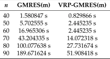
When m = 10, Equation (13) is solved by the GMRES(m) algorithm and VRP-GMRES(m) algorithm, respectively. With the increase of the computational scale, there are few changes in the iteration times for the VRP-GMRES(m) algorithm, and it is much lower than that for the GMRES(m) algorithm, as shown in Figure5a. Thus, the new algorithm has higher computational efficiency. At the same time, it has higher computational accuracy, as is shown in Figure5b. In addition, the total computation time for the VRP-GMRES(m) algorithm is much less than that for the GMRES(m) algorithm, as is shown in Table5.
40 50 60 70 80 90
10 110 210 310 310 n iteration number GMRES(m) VRP−GMRES(m)
(a)
40 50 60 70 80 90
2 4 6 8 10 12 12x 10
−9
n
||b−Ax||
GMRES(m) VRP−GMRES(m)
(b)
Figure 5. Comparison of the computational efficiency and accuracy under different meshes for the two algorithms (m = 10). (a) comparison of computational efficiency; and (b) comparison of computational accuracy.
Table 5.Comparison of computation times under different meshes for the two algorithms (m=10).
n GMRES(m) VRP-GMRES(m)
40 1.580847 s 0.829866 s
50 5.702555 s 2.445235 s
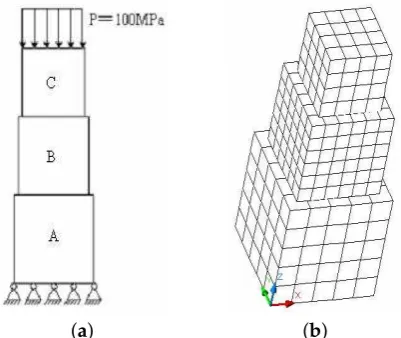
Example 3. Consider an elastic body A, B, C (with sides of 5mm, 4mm, 3mm) in contact with each other. The model and the discrete meshes are shown in Figure6. The discrete data are shown in Table 6. Bodies A, B and C are of the same material with Young modulusE=210GpaPoisson ratioυ= 0.3, and the friction coefficient f = 0.2. For body C, a uniform loadP = 100Mpais applied tothe top surface. The total load is divided into six steps, and the contact tolerance is 0.001mm.
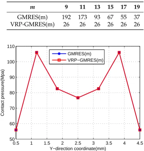
In the example, the VRP-GMRES(m) algorithm is used as a fast solver for the FM-BEM, and some results are shown in Figure7, which are consistent with those obtained by the GMRES(m) algorithm. The iteration times by the GMRES(m) algorithm and VRP-GMRES(m) algorithm are shown in Table 7. From Table7, we can see that there are few changes in the iteration times for the VRP-GMRES(m) algorithm. However, the relative error is quite small for the pressure of the same node, as is shown in Figure8.
(a) (b)
Figure 6.Calculation model and discrete meshes.
Table 6.Discrete data.
Body A Body B Body C Sum
Node number 152 218 98 468
Element number 150 216 96 462
Contact nodes 36 49 25 110
Contact elements 25 36 16 77
0 1
2 3
4 5
0 1 2 3 4 5 −2.5 −2 −1.5 −1 −0.5
x 10−3
Contact width (mm)
Contact length (mm)
Displacements (mm)
Figure 7.Displacements on the contact surface for body A (z=5 mm).
Table 7.Comparison of iteration times for the two algorithms.
m 9 11 13 15 17 19
GMRES(m) 192 173 93 67 55 37
VRP-GMRES(m) 26 26 26 26 26 26
0.5 1 1.5 2 2.5 3 3.5 4 4.5
50 60 70 80 90 100 110
Y−direction coordinate(mm)
Contact pressure(Mpa)
GMRES(m) VRP−GMRES(m)
Figure 8.Comparison of pressure using two algorithms (x=2.5 mm,z=5 mm).
From Table7and Figure8, the VRP-GMRES(m) algorithm is more rapidly and stably convergent than the GMRES(m) algorithm .
5. Conclusions
efficient and rapidly convergent for the elastic problems. On the whole, the new algorithm has extensive prospects in the FM-BEM field and other large-scale scientific and engineering computing.
Acknowledgments:This work is supported by National Natural Science Foundation of China (No. 11301459) and Natural Science Foundation of Hebei Province (No. A2015203121).
Conflicts of Interest:The authors declare no conflict interest.
References
1. Greengard, L.; Rokhlin, V. A fast algorithm for particle simulations.J. Comput. Phys. 2001,73, 325–348. 2. Rokhlin, V. A fast algorithm for the discrete Laplace transformation.J. Complex. 1988,4, 12–32.
3. White, C.A.; Head-Gordon, M. Derivation and efficient implementation of the fast multipole method.
J. Chem. Phys. 1994,101, 6593–6605.
4. White, C.A.; Johnson, B.G.; Gill, P.M.W.; Head-Gordon, M. The continuous fast multipole method.
Chem. Phys. Lett.1994,230, 8–16.
5. White, C.A.; Head-Gordon, M. Rotating around the quartic angular momentum barrier in fast multipole method calculations.J. Chem. Phys. 1996,105, 5061–5067.
6. Beatson, R.; Greengard, L.A Short Course on Fast Multipole Methods. Wavelets Multilevel Methods&Elliptic Pdes; Oxford University Press: Oxford, UK, 1997.
7. Cheng, H.; Greengard, L.; Rokhlin, V. A Fast Adaptive Multipole Algorithm in Three Dimensions.
J. Comput. Phys.1999,155, 468–498.
8. Gu, Y.; Chen, W.; Gao, H.; Zhang, C. A meshless singular boundary method for three-dimensional elasticity problems.Int. J. Numer. Methods Eng.2016,107, 109–126.
9. Wang, Z.; Gu, Y.; Chen, W. Fast-multipole accelerated regularized meshless method for large-scale isotropic heat conduction problems .Int. J. Heat Mass Transf.2016,101, 461–469.
10. Shen, L.; Liu, Y.J. An adaptive fast multipole boundary element method for three-dimensional acoustic wave problems based on the Burton-Miller formulation.Comput. Mech.2007,12, 554–561.
11. Wang, H.; Yao, Z. Large Scale Analysis of Mechanical Properties in 3-D Fiber-Reinforced Composites Usinga New Fast Multipole Boundary Element Method.J. Tsinghua Univ. (Sci. Technol.)2007,12, 461–472.
12. Wang, H.; Yao, Z. Application of a new fast multipole BEM for simulation of 2D elastic solid with large number of inclusions.Acta Mech. Sin. 2004,20, 613–622.
13. Liu, Y.Fast Multipole Boundary Element Method: Theory and Applications in Engineering; Cambridge University Press: Cambridge, UK, 2009.
14. Engheta, N.; Murphy, W.D.; Rokhlin, V.; Vassiliou, M.S. The fast multipole method (FMM) for electromagnetic scattering problems.IEEE Trans. Antennas Propag.1992,40, 634–641.
15. Liu, Y.J.; Nishimura, N.; Yao, Z.H. A fast multipole accelerated method of fundamental solutions for potential problems .Eng. Anal. Bound. Elem.2005,29, 1016–1024.
16. Greengard, L.; Rokhlin, V. A fast algorithm for particle simulations.J. Comput. Phys.2001,73, 325–348. 17. Philippeon, B.; Reichel, L. The generation of Krylov subspace bases.Appl. Numer. Math.2012,62, 1171–1186. 18. Luo, D.M.; Chen, P.J.; Wu, X.M. Application of GMRES algorithm to hovering rotor simulation.
Kongqi Donglixue Xuebao/Acta Aerodyn. Sin.2012,30, 471–476.
19. Dai, Y.Z.; Song, J.Z.; Ren, H.L.; Li, H. Application of GMRES to the hydroelastic analysis of large ofshore structure.Ocean Eng.2003,21, 15–22.
20. Pu, B.Y.; Huang, Y.Z.; Wen, C. A preconditioned and extrapolation-accelerated GMRES method for PageRank.
Appl. Math. Lett.2014,37, 95–100.
21. Saad, Y.; Schultz, M.H. GMRES a Generalized Minimal Residual Algorithm for Solving Non-symmetric Linear Systems.Siam J. Sci. Stat. Comput.2006,7, 856–869.
22. Ayachour, E.H. A fast implementation for GMRES method.J. Comput. Appl. Math.2003,159, 269–283. 23. Jose, E.P.; Alex, A.P.; Ricardo, P.; Carlos, P.P. Making use of BDE-GMRES methods for solving short and
long-term dynamics in power systems.Int. J. Electr. Power Energy Syst.2013,45, 293–302.
25. Lin, F.R.; Yang, S.W.; Jin, X.Q. Preconditioned iterative methods for fractional diffusion equation.
J. Comput. Phys. 2014,256, 109–117.
26. Liang, Y.; Szularz, M.; Yang, L.T. Finite-element-wise domain decomposition iterative solvers with polynomial preconditioning.Math. Comput. Model.2013,58, 421–437.
27. Baker, A.H.On Improving the Performance of the Linear Solver Restarted Gmres; University of Colorado at Boulder: Boulder, CO, USA, 2003.
28. Baker, A.H.; Jessup, E.R.; Kolev, T.V. A simple strategy for varying the restart parameter in GMRES(m).
J. Comput. Appl. Math.2009,230, 751–761.
29. Peairs, L.; Chen, T.Y. Using reinforcement learning to vary the m in GMRES(m).Procedia Comput.2011,4, 2257–2266.
30. Essai, A. Weighted FOM and GMRES for solving nonsymmetric linear systems.Numer. Algorithms1998,18, 227–292.
31. Cai, D.Y.; Bai, F.S.Advanced Numerical Analysis; Tsinghua University Press: Beijing, China, 1997.
c