Heterogeneous Distributed Big Data Clustering on
Sparse Grids
David Pfander1, Gregor Daiß2and Dirk Pflüger3
1 University of Stuttgart; [email protected] 2 University of Stuttgart; [email protected] 3 University of Stuttgart; [email protected]
Version February 1, 2019 submitted to Preprints
Abstract: Clustering is an important task in data mining that has become more challenging due to the 1
ever-increasing size of available datasets. To cope with these big data scenarios, a high-performance 2
clustering approach is required. Sparse grid clustering is a density-based clustering method that 3
uses a sparse grid density estimation as its central building block. The underlying density estimation 4
approach enables the detection of clusters with non-convex shapes and without a predetermined 5
number of clusters. In this work, we introduce a new distributed and performance-portable variant 6
of the sparse grid clustering algorithm that is suited for big data settings. Our compute kernels 7
were implemented in OpenCL to enable portability across a wide range of architectures. For 8
distributed environments, we added a manager-worker scheme that was implemented using MPI. In 9
experiments on two supercomputers, Piz Daint and Hazel Hen, with up to 100 million data points 10
in a 10-dimensional dataset, we show the performance and scalability of our approach. The dataset 11
with 100 million data points was clustered in 1198 s using 128 nodes of Piz Daint. This translates 12
to an overall performance of 352 TFLOPS. On the node-level, we provide results for two GPUs, 13
Nvidia’s Tesla P100 and the AMD FirePro W8100, and one processor-based platform that uses Intel 14
Xeon E5-2680v3 processors. In these experiments, we achieved between 43% and 66% of the peak 15
performance across all compute kernels and devices, demonstrating the performance portability of 16
our approach. 17
Keywords:clustering; machine learning; distributed computing; performance portability; GPGPU; 18
OpenCL; peak performance 19
1. Introduction 20
In data mining, cluster analysis partitions a dataset according to a given measure of similarity. 21
The partitions obtained as a result of the clustering process are called clusters. The clustering of 22
big datasets poses additional challenges as not all clustering algorithms scale well in the size of the 23
dataset. Furthermore, mapping clustering approaches to modern hardware platforms such as graphics 24
processing units (GPUs) requires new parallel approaches. And for the use on supercomputers or in 25
the cloud, algorithms need to be designed for distributed computing. 26
There is a wide range of algorithms that perform clustering. The classic k-means algorithm 27
iteratively improves an initial guess of cluster centers [1]. Efficient variants of thek-means algorithm 28
have been proposed,e.g. by using domain partitioning throughk-d-trees [2] or by a more careful 29
selection of the initial cluster centers [3]. As a major disadvantage, k-means requires the number 30
of clusters to be known in advance, which is not always possible. Moreover, in contrast to many 31
alternativesk-means cannot detect clusters with non-convex shape. 32
DBSCAN probably is the most widely-used density-based clustering approach [4]. In its basic 33
form, it constructs a cluster based on the number of data points in ane-sphere around each data point. 34
If spheres overlap and have enough data points in them, the data points are part of the same cluster. 35
Formdata points, the complexity of DBSCAN was stated asO(mlogm)in the original paper [4]. 36
However, more recent work shows that the actual complexity has a lower bound ofΩ(m4/3)[5,6]. 37
DENCLUE is another example for clustering based on density estimation. It uses a kernel density 38
estimation algorithm [7]. Spectral clustering methods cluster datasets by solving a mincut problem on 39
a weighted neighborhood graph [8]. There are many more approaches to clustering,e.g. using neural 40
networks [9], described in the literature [1,10]. 41
Some clustering algorithms support GPUs for higher performance. Takizawa and Kobayashi 42
presented a distributed and GPU-acceleratedk-means implementation in 2006, before modern GPGPU 43
frameworks like CUDA and OpenCL were available [11]. Since then, further GPU-enabledk-means 44
algorithms have been developed [12–15]. Fewer published results are available for density-based 45
GPU-accelerated clustering. CUDA-DClust is a GPU-accelerated variant of DBSCAN that uses an 46
indexing approach to reduce distance calculations [16]. Andradeet al. developed a GPU-accelerated 47
variant of DBSCAN called G-DBSCAN employing an algorithm with quadratic complexity in the 48
dataset size [17]. 49
While many clustering algorithms have been proposed, not many have been shown to work in 50
big data scenarios.k-means++ is a map-reduce variant of thek-mean algorithm that has been used to 51
cluster a 4.8 million data points dataset on a Hadoop cluster with 1968 nodes [18]. MR-DBSCAN is a 52
DBSCAN variant that could cluster a 2d dataset with up to 1.9 billion data points and is implemented 53
with a map-reduce approach as well [19]. The published results of MR-DBSCAN demonstrate excellent 54
performance. However, it uses a grid discretization that makes assumptions on the distribution of 55
the dataset throughout the domain. Furthermore, it is unclear how the algorithm will scale to higher 56
dimensions, as the grid discretization is fully affected by the curse of dimensionality [20]. RP-DBSCAN 57
implements a similar approach compared to MR-DBSCAN, but uses a more advanced partitioning 58
scheme [5]. RP-DBSCAN was able cluster a 13d dataset with 4.4 billion data points. 59
In this work, we introduce a new distributed and performance-portable variant of the sparse grid 60
clustering algorithm. This approach builds upon prior work which presented the basic theory and 61
compared our approach to other clustering strategies [21]. 62
The unique building block of our approach is the sparse grid density estimation algorithm. Sparse 63
grids are a method for spatial discretization that has been applied to higher-dimensional settings with 64
up to 166 dimensions and moderate intrinsic dimensionality [22]. Therefore, in contrast to many 65
spatial partitioning approaches, the underlying sparse grid density estimation mitigates the curse of 66
dimensionality. The sparse grid clustering method does not rely on assumptions about the distribution 67
of data, it can successfully suppress noise and it can detect clusters of non-convex shape. Compared to 68
k-means, sparse grid clustering does not require the number of clusters as a parameter of the algorithm. 69
In this paper, we use the Euclidean norm as the measure for the similarity of data points. 70
Methods based on sparse grids have been used for regression and classification tasks [22,23]. 71
In prior work, we have shown the applicability of these methods in heterogeneous computing and 72
high-performance computing settings [24–26]. However, to our knowledge this work presents the first 73
high-performance results for sparse grid clustering. 74
Our algorithm was designed with a focus on high performance and performance portability. On 75
the node-level we use OpenCL, as it offers basic portability across a wide range of hardware platforms. 76
We not only support GPUs and processors of different vendors, our approach achieves a major fraction 77
of the peak performance of all devices used. To map our method to clusters and supercomputers, 78
we implemented a distributed manager-worker scheme. Due to the underlying method and the 79
high-performance distributed approach, we show that sparse grid clustering is well-suited for large 80
datasets. We provide results for 10d datasets with up to 100 million data points and 100 clusters. 81
The remainder of this paper is structured as follows. In Sec.2, we give an overview of the 82
sparse grid clustering algorithm. Then, in Sec.3, we introduce the sparse grid density estimation 83
as our core component. The other components of the algorithm are introduced in Sec.4. Section5 84
describes the parallel and distributed implementation and discusses features of the algorithms from 85
0.0 0.2 0.4 0.6 0.8 1.0 0.0
0.2 0.4 0.6 0.8 1.0
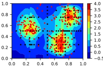
(a)The dataset for cluster analysis
0.0 0.2 0.4 0.6 0.8 1.0 0.0
0.2 0.4 0.6 0.8 1.0
−0.5 0.0 0.5 1.0 1.5 2.0 2.5 3.0 3.5 4.0
(b)A density estimation of the 2d dataset and the grid points (black) of the sparse grid density function
0.0 0.2 0.4 0.6 0.8 1.0 0.0
0.2 0.4 0.6 0.8 1.0
−0.5 0.0 0.5 1.0 1.5 2.0 2.5 3.0 3.5 4.0
(c)After calculating thek-nearest-neighbor graph
0.0 0.2 0.4 0.6 0.8 1.0 0.0
0.2 0.4 0.6 0.8 1.0
−0.5 0.0 0.5 1.0 1.5 2.0 2.5 3.0 3.5 4.0
(d)Thek-nearest-neighbor graph after being pruned
Figure 1. The application of the sparse grid clustering algorithm to a 2d dataset with three slightly overlapping clusters. After calculating the sparse grid density estimation and thek-nearest-neighbor graph, the graph is pruned using the density estimation. This splits the graph into three connected components.
supercomputers in Sec.6. Finally, in Sec.7, we remark on implications of the presented algorithm and 87
discuss future work. 88
2. Clustering on Sparse Grids 89
In this section, we describe the sparse grid clustering algorithm on a high level. We describe its 90
components in Sec.3and4in more detail. 91
Sparse grid clustering assumes ad-dimensional datasetTwithmdata points that was normalized to the unit hypercube[0, 1]d:
T :={xi ∈[0, 1]d}mi=1. (1) We further assume that the dataset has been randomized.
92
The sparse grid clustering algorithm is a four step algorithm. Except for the last one, these steps are 93
shown in Fig.1at the example of a 2d dataset with three clusters. The sparse grid clustering algorithm 94
first calculates a density estimation of the dataset using the sparse grid density estimation algorithm 95
(Fig.1b). Then, ak-nearest-neighbor graph of the dataset is computed (Fig.1c). In the third step, the 96
density estimation is used to prune the graph. The algorithm prunes nodes in low-density regions and 97
edges that intersect low-density regions (Fig.1d). In the fourth and final step the weakly-connected 98
components of the pruned graph are retrieved. The connected components of the graph are returned 99
as the detected clusters. 100
This description immediately suggests one of the tuning parameters of the algorithm. The sparse 101
grid clustering method requires a carefully chosen threshold valuet that is used for pruning the 102
ϕ
3,1ϕ
3,2ϕ
3,3ϕ
3,4ϕ
3,5ϕ
3,6ϕ
3,70 1
(a)A 1d full grid in nodal basis
ϕ
3,1ϕ
2,1ϕ
3,3ϕ
1,1ϕ
3,5ϕ
2,3ϕ
3,70 1
(b)A 1d sparse grid in the hierachical basis
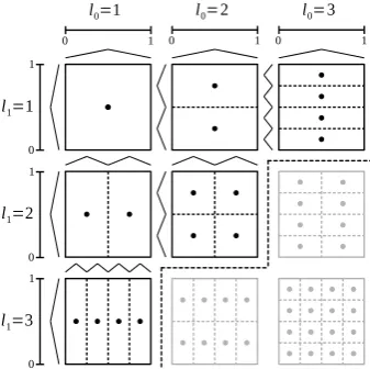
Figure 2.The nodal and the sparse grid in Fig.2aand Fig.2bboth have discretization levell=3 and are equal ford=1. Both use hat functionsφl,ias basis functions, but in a nodal and in a hierarchical
formulation. Note that sparse grids employ less grid points compared to full grids of the same level for d≥2 (see Fig.3).
l0=1 l0=2 l0=3
l1=1
l1=2
l1=3 0 1
0 1
0 1
0 1 0 1 0 1
(a)The subgrids of varying discretization level. Dotted lines outline the support of the basis functions centered at the grid points.
0 1
0 1
(b) The 2d sparse grid (black) obtained by superimposing the components grids.
Figure 3. The subgrids of a sparse grid withl =3 (Fig.3a) and the resulting sparse grid (Fig.3b). Greyed out subgrids and grid points would be part of the corresponding full grid.
3. Estimating Densities on Sparse Grids 104
The sparse grid density estimation is build upon the concept of sparse grids. We therefore briefly 105
introduce sparse grids and then describe how densities can be estimated with the sparse grid method. 106
3.1. Sparse Grids 107
As this work focuses on the sparse grid clustering algorithm and not on the basic sparse grid 108
method, this introduction to sparse grids is necessarily brief. For a thorough presentation, we 109
recommend the overview by Bungartz and Griebel [27]. 110
Ad-dimensional grid can be defined on the unit hypercube[0, 1]dwith an equidistant mesh width 111
hn=2−nfor a discretization levelnand, therefore, 2ndgrid points. With basis functions centered at 112
the grid points, a corresponding function space is spanned by the linear combinations of the basis 113
functions. We call this a full grid approach. Full grids can be represented in a hierarchical basis. From 114
this representation, it is a small step to sparse grids. 115
The hierarchical approach constructs a final grid by superimposing a set of subgrids. First, we define an index set that is used to enumerate the grid points on thed-dimensional subgrids of discretization levell∈Nd:
Il:={(i1, . . . ,id): 0<ik <2lk,ikodd}. (2) In this work, we employ hat functions as basis functions. The scaled and translated 1d hat functions are defined as
Ford>1, we use a tensor-product approach:
φl,i(x):= d
∏
j=1φlj,ij(xj). (4)
Given an index setIland the basis functionsφl,i, we can define the subspaces
Wl:=span{φl,i:i∈Il}. (5) The subgrids and their grid points xl,i := (i1hl1, . . . ,idhld) for the subspaces W(1,1). . .W(3,3) are
116
displayed in Fig.3afor a 2d grid. 117
With the direct sumL
, a full grid of discretization leveln∈ Nin the hierarchical basis can be
defined as
Vn:=
M
|l|∞≤n
Wl. (6)
Figure2shows how a 1d grid is represented in the standard (nodal) basis (Fig.2a) and the hierarchical 118
basis (Fig.2b). 119
Sparse grids are based on the observation that for sufficiently smooth functions only a small additional interpolation error is introduced if certain grid points are removed [27]. This mitigates the curse of dimensionality. As a result, the sparse grid function spaceVn(1)is constructed from a different set of subspaces:
Vn(1):=
M
|l|1≤n+d−1
Wl. (7)
Figure3shows how a 2d sparse grid is constructed from subgrids that correspond to the subspaces of 120
the grid. 121
A sparse grid function f ∈Vn(1)is given as
f(x) =
∑
|l|1≤n+d−1i
∑
∈Ilαl,iφl,i(x) =: N
∑
j=1αjφj(x), (8)
where we sum up allNweighted basis functions in some order, and whereNdenotes the total number 122
of grid points. Since our algorithms iterate the basis functions linearly, we use the simplified notation 123
when the algorithms are presented. The coefficientsαl,iare usually referred to as surpluses. 124
3.2. The Sparse Grid Density Estimation 125
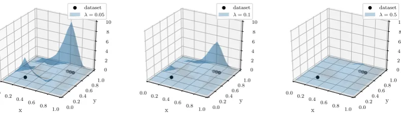
The sparse grid density estimation, originally proposed by Heglandet al. [28], uses an initial density guessfethan is smoothed using a spline-smoothing approach:
ˆ
f =arg min u∈V
Z
Ω(u(x)− fe(x)) 2dx+
λ||Lu||2L2. (9)
This approach results in a function ˆf ∈ Vthat balances closeness to the initial density guess with the regularization term||Lu||2
L2 that enforces smoothness on the resulting density function. The
regularization parameterλcontrols the degree of smoothness of ˆf. Lusually is some differential operator. We use the initial density guess proposed by Heglandet al. that places a Dirac delta function δxiat every data pointxi:
fe:=
1 m
m
∑
i=1x
0.0 0.2 0.4
0.6 0.8
1.0
y
0.00.2 0.40.6
0.81.0 0 2 4 6 8 10 dataset
λ= 0.05
x
0.0 0.2 0.4
0.6 0.8
1.0
y
0.00.2 0.40.6
0.81.0 0 2 4 6 8 10 dataset
λ= 0.1
x
0.0 0.2 0.4
0.6 0.8
1.0
y
0.00.2 0.40.6
0.81.0 0 2 4 6 8 10 dataset
λ= 0.5
Figure 4.The effect of the regularization parameterλon a 2d dataset with four data points. For smaller λvalues, the function becomes more similar to the initial density guess of Diracδfunctions. The function becomes smoother for higher values ofλ.
As in prior work, we compute the best sparse grid functionu ∈Vn(1)and use a surplus-based regularization approach [22]. Therefore, the problem to solve is
ˆ
f =arg min u∈Vn(1)
Z
Ω(u(x)−fe(x)) 2dx+
λ N
∑
i=1α2i. (11)
This formulation leads to a system of linear equations
(B+λI)α=b, (12)
withBij= (φi,φj)L2, the identity matrixIandbi =
1
m∑mj=1φi(xj). 126
We solve this system of linear equations with a conjugate gradient solver (CG). Given this iterative solver, two major operations need to be performed: calculating the right-hand side once and computing the matrix-vector productv0= (B+λI)vin every CG iteration. The calculation of the right-hand side is straightforward. However, the matrix-vector product requires efficient computations of theL2inner product of pairs of basis functions:
(φl,i,φl0,i0)L
2 = Z
Ωφl,i(x)φl0,i0(x)dx (13) =
Z 1
0 φl1,i1(x1)φl 0
1,i01(x1)dx1· · ·
Z 1
0 φld,id(xd)φl 0
d,i0d(xd)dxd. (14)
The 1d integrals can be computed directly:
Z 1
0 φl,i(x)φl
0,i0(x)dx=
(2
3hl, xli=xl0i0, hl0φl,i(xl0i0) +hlφl0i0(xli), else.
(15)
We note that in many instances the integral will be zero due to the non-overlapping support of the hat 127
functions. 128
Figure4shows the effect of varying the regularization parameterλfor a 2d dataset.λhas to be 129
chosen with care, as too small values might split a single cluster into multiple clusters. On the other 130
hand, ifλis too large separate clusters could be part of the same high-density region. 131
3.3. Streaming Algorithms for the Sparse Grid Density Estimation 132
A high-performance sparse grid density estimation algorithm needs to efficiently compute the 133
two operations described above: the computations of the matrix-vector productv0 = (B+λI)vand the 134
right-hand sidebwithbi= m1 ∑m
j=1φi(xj). To efficiently perform these operations, we use an implicit 135
This approach might seem wasteful at first glance. However, as the size ofBscales quadratically in the 137
number of grid points, it quickly becomes infeasible to store the matrix in memory. 138
Algorithm 1:The streaming algorithm for computing the right-hand sideb
fori=0 . . .Ndo bi←0
forj=0 . . .mdo bi+=∏dimd=1φ
(d) i (x
(d) j )
bi← m1bi
Algorithm 2:The streaming algorithm for computing the matrix-vector multiplication v0= (B+λI)v
fori=0 . . .Ndo v0i ←0
forj=0 . . .Ndo v0i +=∏dim
d=1 R1
0 φ (d) i φ
(d) j dx·vj v0i +=λ·vi
139
The computation of the right-hand side requires the computation of mvector components. 140
Algorithm1shows the loop structure of a scalar version of this operation. As the basis function 141
evaluations in the innermost loop are independent, we can parallelize this algorithm over the outer 142
loop,i.e. the iteration over the grid points. The evaluation of hat functions is branch-free. Therefore, 143
this algorithm is well-suited for vectorization. 144
We can formulate the matrix-vector operation as a second streaming algorithm with two nested 145
loops over the grid points. This is shown in Algorithm2. Similar to the hat function evaluations of 146
the right-hand side, theL2norms can be independently computed as well. Thus, we can parallelize 147
Algorithm2by processing the outer loop in parallel. The two cases for computing the 1d integral 148
according to Eq.15slightly complicate vectorization. Our approach is the computation of both cases 149
in a vectorized algorithm and a single conditional move to return the correct result. Computing 150
thexli = xl0i0 case is only a single multiplication, as we can move the computation ofhl = 2−l to 151
a precomputation step. Therefore, and because the xli = xl0i0 case rarely occurs, the overhead in 152
each integration step is low compared to an optimal algorithm that would only evaluate the correct 153
integration case. 154
4. Other Steps 155
In this section, we first present the algorithm for computing thek-nearest-neighbor graph. Then, 156
we show how we apply the sparse grid density estimation to prune it. Finally, we briefly describe how 157
we perform the connected component search in the pruned graph. 158
4.1. Computing the k-Nearest-Neighbor Graph 159
Algorithm 3:A variant of theO(m2)k-nearest-neighbor algorithm that usesbbins. Input : datasetT={xi∈[0, 1]d}m
i=1
Output : k-nearest-neighbor graphgas neighborhood list forc=1 . . .bdo
distsc←0 fori=1 . . .mdo
c←0// c iterates over the number of bins forj=1 . . .mdo
dist←distance(xi,xj) ifdist<distsc+1then
binsc+1←j distsc+1←dist c←(c+1)modb
To create thek-nearest-neighbor graph, we have developed an approximate variant of theO((k+ 160
d)m2)algorithm that compares all pairs of data points. Instead of creating a neighborhood list with 161
kentries directly, we employ an approach withbbins that implicitly splits the dataset intobranges. 162
For every data pointithe dataset is iterated. Thereafter, each bin contains the nearest neighbor of its 163
assigned range of data points. To obtain an approximatek-nearest-neighbor solution, thekindices 164
with the smallest associated distances are selected from thebbins. Pseudocode for this approach is 165
displayed in Algorithm3. 166
Thisk-nearest-neighbor algorithm offers several advantages. It is not affected by the curse of 167
dimensionality and therefore works well for the higher-dimensional datasets we target. In contrast, 168
spatial partitioning approaches such as k-d-trees tend to suffer from the curse of dimensionality. 169
Furthermore, it maps well to modern hardware architectures as it is straightforward to parallelize and 170
vectorize. Through cache blocking of the outer loop that iteratesi, the resulting algorithm is highly 171
cache-efficient as well. Finally, the number of binsbis the only parameter to specify. 172
Binning was introduced for performance reasons. It allows us to only perform a single comparison 173
in the innermost loop instead ofkcomparisons and, therefore, reduces the complexity toO(dm2). The 174
effect on the detected clusters is minimal, as it is very likely that nodes are still connected to close-by 175
nodes of the same density region and therefore the same cluster. Furthermore, edges that intersect 176
low-density regions get pruned, as we describe in the next section. 177
The overall clustering algorithm is relatively robust with regard to different values ofk. However, 178
kshould not be too small. Otherwise, thek-nearest-neighbor graph might be split into more connected 179
components than are desired. For larger values ofk, performance decreases slightly in the subsequent 180
pruning step as the pruning algorithm has linear complexity ink. In our experience, choosingkwith 181
values between five and ten balances this trade-off. Consequently, we setbto 16, as it is larger than 182
expected values ofkand leads to a good-enough approximation of thek-nearest-neighbor graph. 183
On modern hardware platforms, this choice ofbshould not increase the cache or register memory 184
requirements of the algorithm to an extent that would affect performance. 185
4.2. Pruning the k-Nearest-Neighbor Graph 186
Algorithm 4: A streaming algorithm for pruning low-density nodes and edges of the k-nearest-neighbor graph. The density function is evaluated at the location of the nodes and at the midpoints of the edges.
Input : k-nearest-neighbor graphgas neighborhood list, datasetT, density estimation ˆf(x) =∑N
j αjφj(x), thresholdt Output : prunedk-nearest-neighbor graphg
fori=0 . . .mdo iffˆ(xi)<tthen
prune_node(gi) continue
p1, . . . ,pk←load_midpoints(T,gi) forj=1 . . .kdo
iffˆ(pj)<tthen prune_edge(gi,j)
To prune thek-nearest-neighbor graph, we use two criteria. The density function is evaluated at 187
the positionxithat corresponds to the current graph nodegi. If the density is below a thresholdt, the 188
node and its edges are removed. Furthermore, we evaluate at the midpoints of all outgoing edges and 189
prune all edges where the density is belowt. By evaluating the midpoints, clusters can be successfully 190
separated even if two data points are in high-density regions that belong to different clusters. Our 191
Similar to the other algorithms presented, iterations of the outer loop are independent and can 193
therefore be parallelized. The most expensive operations in this loop, multiple evaluations of the 194
density function, are branch-free. Therefore, this algorithm is straightforward to vectorize as well. 195
As there are only O(m·(k+1)) conditionals compared to overallO(m(k+1)N) operations, the 196
conditionals do not significantly impact performance. 197
4.3. Connected Component Detection 198
To detect the weakly connected components in the pruned graph, we first convert the directed 199
graph to an undirected graph by adding all inverted edges. Then, we perform a depth-first search 200
to detect the connected components. This classical algorithm performsO(km)memory operations. 201
Because the complexity of this algorithm is significantly lower compared to all other steps, this 202
algorithm is only shared-memory parallelized and not distributed. 203
5. Implementation 204
In this section, we describe how our sparse grid clustering approach was implemented. To that 205
end, we first consider the OpenCL-based node-level implementation and then present our distributed 206
manager-worker approach. 207
5.1. Node-Level Implementation 208
Except for the connected component detection, all steps of the clustering algorithm have been 209
implemented as OpenCL kernels. There are two OpenCL kernels for the density estimation: one for 210
calculating the right-hand side and one for the matrix-vector multiplication. A third OpenCL kernel 211
implements thek-nearest-neighbor graph creation and a fourth kernel implements the density-based 212
graph pruning. 213
From a performance engineering perspective, these OpenCL kernels have some commonalities. 214
All kernels were parallelized over the outermost loop, exploiting the fact that the loop iterations are 215
independent. Furthermore, all OpenCL kernels were designed to be branch-free. The only exception is 216
the density matrix-vector multiplication kernel that has a single branch in the innermost loop. This 217
branch is implemented using the OpenCLselectfunction to differentiate between the integration cases. 218
On modern OpenCL platforms, this should be compiled to a conditional move. Because only standard 219
arithmetic is used and because of the regular control flow, the four compute kernels get vectorized on 220
all OpenCL platforms we tested. Due to the design of the compute kernels, we expect this to be the 221
case on many untested OpenCL platforms as well. 222
The local memory is used in all kernels to either share grid points or data points between all 223
threads of the work-group. For example, the prune graph kernel evaluates 1d sparse grid basis 224
functions in its innermost loop. The threads of a work-group process different data points, but all 225
always evaluate their data point with the same basis function. Therefore, the data of the currently 226
processed basis function can be shared efficiently through the local memory. Furthermore, the data 227
point assigned to a thread remains constant throughout the lifetime of the thread. It can therefore be 228
stored inprivatememory, which translates to the register file on GPU devices and the L1 cache (or the 229
registers) on processors. 230
Table1shows the number of floating-point operations for the different OpenCL kernels. As both 231
the number of grid pointsNand the size of the datasetmcan be large, all operations are potentially 232
expensive. In most data mining scenarios, the sparse grid will have significantly fewer grid points 233
than there are data points. Therefore, thek-nearest-neighbor graph creation is expected to be the most 234
expensive operation. Depending on the number of CG iterations, the density matrix-vector product 235
can be moderately expensive as well. However, it only depends on the grid points and therefore 236
benefits fromN<m. 237
To estimate the achievable performance of our compute kernels, we calculated the arithmetic 238
Kernel FP ops./complexity Arith. int. (ws=1) Arith. int. (ws=128) Peak lim. (%)
density right-hand side N·m·d·6 1.5 F B−1 192 F B−1 67%
density matrix-vector CG-iter.·N2·d·14 1.2 F B−1 149 F B−1 64%
create graph m2·d·3 1.0 F B−1 129 F B−1 83%
prune graph m·N·(k+1)·d·6 4.5 F B−1 576 F B−1 67%
Table 1.The number of floating-point operations for the different OpenCL kernels and the arithmetic intensities (in floating point operations per byte) for a work-group size (ws) of one thread and 128 threads. The peak limit states the achievable fraction of the peak performance given the instruction mix of the compute kernels.
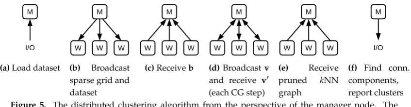
I/O M
(a)Load dataset
M
W W W
(b) Broadcast sparse grid and dataset
M
W W W
(c)Receiveb
M
W W W
(d)Broadcastv
and receive v0
(each CG step)
M
W W W
(e) Receive
pruned kNN
graph
I/O M
(f) Find conn. components, report clusters
Figure 5. The distributed clustering algorithm from the perspective of the manager node. The (inexpensive) assignment of index ranges is not shown.
single thread would be too low to achieve a significant fraction of the peak performance on modern 240
hardware platforms (see Tab.2for the machine balances of the hardware platforms we used). However, 241
with a larger work-group size of 128 threads, and because we efficiently use the shared memory, 242
the arithmetic intensity is strongly improved. As a consequence, memory accesses do not limit the 243
performance of these compute kernels on modern hardware platforms. On processor-based platforms, 244
the L1 cache enables similarly-high arithmetic intensity values. 245
The arithmetic intensity values would allow our compute kernels to achieve peak performance. 246
However, as our compute kernels make use of instructions other than fused-multiply-add (FMA) 247
operations, the instruction mix reduces the achievable performance. To calculate the peak limit given 248
in Tab.1, we make the (realistic) assumption that the remaining vector floating-point instructions run 249
at half the performance of the FMA instructions [29]. 250
5.2. Distributed Implementation 251
For distributed computing, we developed a manager-worker model that was implemented with 252
MPI. To create work that can be assigned to the workers, we split the loops that were used for 253
parallelization (the outermost loops of the compute kernels) once again. We use a static load balancing 254
scheme that distributes the work equally to the workers. Our implementation supports single as well 255
as double precision. Currently, we transfer double precision data even if single precision is used in the 256
compute kernels. 257
From the perspective of the manager node, the distributed algorithm consists of four major steps: 258
creating the right-hand side of the density estimation, the density matrix-vector products, an integrated 259
graph-creation-and-prune step and the connected component search. These steps are shown in Fig.5. 260
Note that the matrix-vector multiplication step (Fig.5d) is repeated once per CG iteration. 261
When the application is started, the dataset is read by the manager node and sent to all workers, 262
requiringm·d·8 B of communication per worker. Then, the manager node creates the grid and sends it 263
to the workers as well. This requires 2·N·d·8 B per worker to be communicated. After these relatively 264
expensive transfers are completed, grid and dataset are held by the workers. Therefore, most remaining 265
communication steps only require small amounts of data to be transferred. We demonstrate in Sec.6 266
that the overhead of these communication steps is indeed very low compared to the computational 267
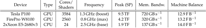
Device Type Cores/
Shaders Frequency Peak (SP) Mem. Bandw. Machine Balance
Tesla P100 GPU 3584 1.3 GHz (boost) 9.5 TF 720 GB s−1 12.9 F B−1
FirePro W8100 GPU 2560 0.8 GHz (max) 4.2 TF 320 GB s−1 13.2 F B−1
2xXeon E5-2680v3 CPU 24 2.5 GHz (base) 1.9 TF 137 GB s−1 14.0 F B−1
Table 2. The hardware platforms used in the distributed and node-level experiments. We list the frequency type that best matches our observations during the experiments.
To compute the density right-hand-side operation, every worker computes an index range of the 269
components ofb. Asbis aggregated on the manager node,N·8 B need to be transferred. During each 270
CG step and after the final CG step, the manager sendsv(αafter the final iteration) to all workers. 271
Each worker calculates the result of an index range ofv0and communicates the partial result back to 272
the manager node. Therefore,N·8 B per worker are communicated during each iteration and after the 273
final iteration. Collecting the partial results forv0requires anotherN·8 B to be transferred per CG 274
step. 275
The creation of thek-nearest-neighbor graph only requires the assignment of index ranges and no 276
further communication. Because the pruning of thek-nearest-neighbor graph reuses the same index 277
ranges that were assigned in the graph creation step, this step only requires the pruned graph to be 278
sent to the manager node. This step requiresk·m·8 B to be transferred. Having received the pruned 279
graph, the manager node performs the connected component detection and has thereby computed the 280
clusters. 281
6. Results 282
In this section, we evaluate our distributed and performance-portable sparse grid clustering 283
approach. We first present the hardware platforms and datasets that were used in the experiments. 284
Then we provide the results of our node-level experiments that demonstrate performance portability. 285
The quality of the clustering is discussed in the context of the node-level experiments as well. Finally, 286
we present distributed performance results for two supercomputers: Hazel Hen and Piz Daint. 287
6.1. Hardware Platforms 288
On the node level, we used three different hardware platforms. Two of them are GPUs: the 289
Nvidia Tesla P100 and the AMD FirePro W8100. To represent standard processor platforms, we used a 290
dual socket machine with two Intel Xeon E5-2680v3 processors. The relevant technical details of these 291
hardware platforms are summarized in Tab.2. 292
Our distributed experiments were conducted on two supercomputers. The Cray XC40 Hazel Hen 293
is an Intel processor-based machine with 7712 nodes for a peak performance of 7.4 PF. Hazel Hen is 294
located at the High Performance Computing Center Stuttgart (HLRS) in Stuttgart, Germany. It has 295
dual socket nodes with Xeon E5-2680v3 processors and 128 GB of memory per node. 296
The Cray XC40/XC50 Piz Daint is a mostly GPU-based supercomputer with a peak performance of 297
27 PF. Piz Daint is located at the Swiss National Supercomputing Centre (CSCS) in Lugano, Switzerland. 298
Each of the XC50 nodes that we used have a single Intel Xeon E5-2690v3 processor with 64 GB of 299
memory and a single Nvidia Tesla P100 GPU. In our experiments, we only used the Tesla P100 to 300
compute the main compute kernels of our application. 301
6.2. Datasets and Experimental Setup 302
In all of our experiments, we used synthetic datasets with clusters drawn from Gaussian 303
distributions. The cluster centersµwere drawn randomly. We normalized the datasets to[0.1, 0.9]d. As 304
this moves data points sufficiently towards the center of the domain, we can use a sparse grid without 305
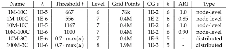
Name Size Clust. σ Dim. Dist. Noise Type
10M-3C 10M 3 0.12 10 3·σ 0% distributed
100M-3C 100M 3 0.12 10 3·σ 0% distributed
1M-10C 1M 10 0.05 10 7·σ 2% node-level
1M-100C 1M 100 0.05 10 7·σ 2% node-level
10M-100C 10M 100 0.05 10 7·σ 2% node-level
Table 3.The Gaussian datasets for the distributed and the node-level runs
Name λ Thresholdt Level Grid Points CGe k ARI Type
1M-10C 1E-5 667 6 76k 1E-2 6 1.0 node-level
1M-100C 1E-6 556 7 0.4M 1E-2 6 0.85 node-level
10M-10C 1E-5 1167 7 0.4M 1E-2 6 1.0 node-level
10M-100C 1E-6 1000 7 0.4M 1E-2 6 0.90 node-level
10M-3C 1E-6 0.7·max(α) 7 0.4M 1E-3 5 - distributed
100M-3C 1E-6 0.7·max(α) 8 1.9M 1E-3 5 - distributed
Table 4.The parameters used for configuring the clustering algorithm and the adjusted Rand index (ARI) for the node-level experiments. In the distributed runs, the threshold was specified as a fraction of the maximum surplus of the density function. The node-level runs used an absolute threshold value.
The parameters used to generate the datasets are listed in Tab.3. The datasets with 100 clusters 307
are challenging, as the density estimation needs to correctly separate 100 high-density regions in a 308
moderately-high dimensional setting. Furthermore, to make it possible to assess the quality of the 309
clustering, we generated the node-level dataset so that the clusters are well-separated by forcing a 310
minimum distance of 7·σbetween the cluster centers. We verified that the noise connects all clusters 311
in the unprunedk-nearest-neighbor graph. 312
As the clustering algorithm requires parameterization as well, these parameters are shown in 313
Tab.4. The adjusted Rand index (ARI) is a quality measure for clustering and is addressed in Sec.6.4. 314
In all of our experiments, we used single-precision floating-point arithmetic. 315
6.3. Node-Level Performance and Performance-Portability 316
The tables6and7show the runtimes of the node-level experiments. For more consistent results, 317
the runs were repeated four times and the measurements averaged. The 1M-10C dataset could be 318
processed on a Tesla P100 in less than 20 s. Processing the 1M-100C dataset is more time-consuming 319
and required 248 s again using a Tesla P100. The main reason for the time increase is because the 320
density estimation requires more time due to a larger sparse grid and a smallerλ, which leads to more 321
CG iterations. 322
Tesla P100 FirePro W8100 2xE5-2680v3
dens. right-hand side GFLOPS 4584 2271 (753 MHz) 1177
limit: 67% peak peak (of lim.) 48% (72%) 59% (88%) 61% (91%)
dens. matrix-vector GFLOPS 4090 1939 (759 MHz) 919
limit: 64% peak peak (of lim.) 43% (67%) 50% (78%) 48% (75%)
create graph GFLOPS 5474 1433 (467 MHz) 852
limit: 83% peak peak (of lim.) 58% (70%) 60% (72%) 44% (53%)
prune graph GFLOPS 5360 1817 (822 MHz) 1265
limit: 67% peak peak (of lim.) 56% (84%) 43% (64%) 66% (99%)
P100 W8100 2xE5-2680v3 0
20 40 60 80
Duration
(s)
1M Data Points, 10 Clusters
dens. right-hand side sum density mult. create graph prune graph
(a)λ=1E−5,l=6,t=667
P100 W8100 2xE5-2680v3
0 200 400 600 800 1000
Duration
(s)
1M Data Points, 100 Clusters
dens. right-hand side sum density mult. create graph prune graph
(b)λ=1E−6,l=7,t=556
Figure 6. The duration of the node-level experiments with one million data points. Because the 1M-100C dataset requires a larger grid, the density estimation takes up most of the overall runtime.
P100 W8100 2xE5-2680v3
0 1000 2000 3000 4000 5000
Duration
(s)
10M Data Points, 10 Clusters
dens. right-hand side sum density mult. create graph prune graph
(a)λ=1E−5,l=7,t=1167
P100 W8100 2xE5-2680v3
0 1000 2000 3000 4000 5000 6000
Duration
(s)
10M Data Points, 100 Clusters
dens. right-hand side sum density mult. create graph prune graph
(b)λ=1E−6,l=7,t=1000
The experiments with the 10 million data points datasets are shown in Tab.7. Due to the increased 323
size of the datasets, thek-nearest-neighbor graph creation takes up the largest fraction of the runtime 324
in both experiments. This illustrates that for large datasets, because of its quadratic complexity, the 325
k-nearest-neighbor graph creation step will dominate the overall runtime. In these two experiments, 326
increasing the number of clusters has only a small effect on the runtime. Mainly, because in both 327
cases a sparse grid with levell = 7 was used. On the P100 platform, the experiments with the 328
10M-100C dataset took 1162 s. The other hardware platforms took longer, proportional to their lower 329
raw performance. 330
Table 5 shows the performance achieved in the node-level experiments. It displays the 331
performance in GFLOPS and the achieved fraction of peak performance. The achieved fraction 332
of the peak performance relative to the instruction-mix-based limit is displayed as well. These results 333
were calculated from the runs with the 10M-10C dataset as specified in Tab.4. 334
Our implementation achieved a significant fraction of the peak performance across all devices. 335
Additionally, if the limit imposed by the instruction mix is taken into account, we see that many 336
combinations of kernels and devices run close to their maximally achievable performance. The only 337
kernel that reaches less than two-thirds of its achievable performance is the create graph kernel on 338
the Xeon E5 platform. We suspect that this is due to throttling of the processor, as this operation puts 339
extreme stress on the vector units. 340
The fastest device by a significant margin is the Tesla P100, as it is the most recent of the devices and 341
has the highest theoretical peak performance. It is 2.23−3.29x faster than the W8100 and 4.41−5.49x 342
faster than the Xeon E5 pair. 343
The FirePro W8100 achieves similar fractions of the peak performance compared to the P100 at a 344
lower absolute level of performance. It is still 1.67−1.98x faster than the pair of Xeon E5 processors. 345
During our experiments, the FirePro W8100 displayed strong throttling which is why we list the 346
average frequencies observed for the invidivual compute kernels. The reduced frequencies imply 347
lower achievable peak performance (2·2560· favr) which we take into account for the calculation 348
of the peak performance and the resulting achieved fraction of peak performance. The average 349
frequencies reported were measured in a separate run of the 10M-10C experiment. In case of the 350
k-nearest-neighbor graph kernel, a frequency of only 492 MHz was measured. This nearly halves the 351
achievable performance of this compute kernel. 352
Because it has the lowest absolute performance, the pair of Xeon E5 processors scores lowest. 353
However, the achieved fractions of the peak performance are similar to the other devices. This indicates 354
that performance is not only portable across GPU platforms, but processor-based platforms as well. 355
6.4. Clustering Quality and Parameter Tuning 356
This work mostly focuses on the performance of our sparse grid clustering approach. Nevertheless, 357
to make our evaluation more realistic, we tuned the clustering parameters of our node-level runs for 358
(nearly) optimal clustering quality. For a more detailed discussion of the achievable level of quality, 359
we refer to prior work which compared sparse grid clustering to other clustering algorithms [21]. A 360
comparison of the sparse grid density estimation to other density estimation methods is available as 361
well [30]. 362
To assess the quality, we used the adjusted Rand index (ARI) which compares two cluster 363
mappings. Because we know the mapping of data points to clusters of each of our synthetic datasets, 364
these reference cluster mappings were compared to the output of the sparse grid clustering algorithm. 365
The calculated ARI of the node-level experiments is shown in Tab.4. These results show that we 366
can nearly perfectly reconstruct the clusters of both datasets with ten clusters. The datasets with 100 367
clusters are more challenging and would require slightly larger grids for further improvements. 368
We used a parameter tuning approach to fit the computed cluster mappings to the reference 369
mappings. During parameter tuning, we first select a value for the regularization parameterλand 370
To speed up parameter tuning in general, our sparse grid clustering implementation allows for 372
reusing of thek-nearest-neighbor graph and calculated density estimations. As thek-nearest-neighbor 373
graph is the same independent of all parameters, it can be calculated once overall. Moreover, the 374
density estimation changes only ifλis changed. Thus, the density estimation can be reused while 375
an optimal value fortis searched. Only the comparably cheap graph pruning operation and the 376
connected component search are performed at every parameter tuning step. 377
6.5. Distributed Results on Hazel Hen 378
Figure8shows the results of the distributed experiments conducted on Hazel Hen. Results are 379
given for the individual compute kernels as well as the whole application run. The total runtime, and 380
the average application TFLOPS derived from it, is based on the wall-clock time of the application and 381
not only on the three major distributed operations. At the highest node count, it took 4226 s to process 382
the 100M-3C dataset and 259 s to process the 10M-3C dataset. We achieved up to 100 TFLOPS for the 383
100M-3C dataset using 128 nodes and up to 23 TFLOPS for the 10M-3C using 32 nodes. Therefore, 384
we achieved 41% and 37% of the peak performance at the highest number of nodes for the whole 385
application including all communication and file input-output operations. 386
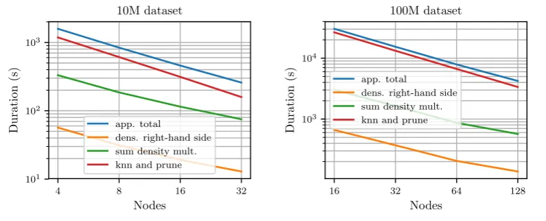
The creation and pruning of thek-nearest-neighbor graph scales nearly linearly. Calculating the 387
density estimation scales slightly worse. As the grid is much smaller than the dataset, there is too little 388
work available per node during the density estimation step to achieve optimal performance at high 389
node counts. 390
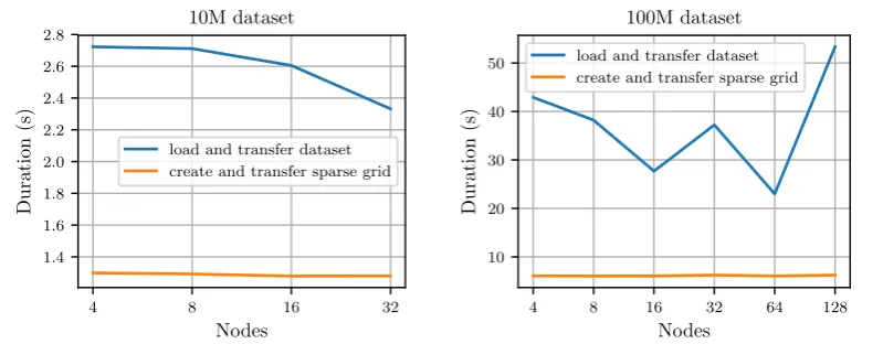
Figure8cdisplays the duration of the initial loading and distribution of the dataset, the creation 391
and the transfer of the sparse grid and the duration of the connected component search. As Fig.8c 392
shows, loading and communicating the dataset does not take up significant amounts of time. The 393
same is true for creating and transferring the sparse grid. However, the connected component search 394
becomes relatively expensive for the 100M-3C dataset, as it is performed on a single node and therefore 395
cannot scale with an increasing number of nodes. Nevertheless, at 128 nodes the connected component 396
search still only requires 107 s or 2.5% of the total runtime for the 100M-3C dataset. For the 10M-3C 397
dataset and 32 nodes, the connected component search takes up 2.2% of the total runtime. 398
6.6. Distributed Results on Piz Daint 399
We conducted the distributed experiments before we were able to do some final node-level 400
optimizations, and due to compute time limitations we were not able to recompute the experiments. 401
Thus, the results of these experiments are not directly comparable to the node-level performance 402
results. Since these experiments, the node-level performance of all compute kernels was improved. 403
Because of this, scalability might by slightly overestimated. Furthermore, the duration of the connected 404
component search is not listed in these results, as we used a different algorithm at the time of the 405
experiments. 406
Figure9shows duration and performance of the experiments performed on Piz Daint for both 407
the 10M-3C and 100M-3C datasets. Again, results are given for the individual compute kernels as well 408
as the whole application run. As Fig.9ashows, the application scales well to 128 nodes. Similar to 409
the Hazel Hen results, the integrated graph-creation-and-prune step scales nearly linearly, whereas 410
the density estimation scales slightly worse. Using 32 nodes, the clustering of the 10M-3C dataset 411
takes 100 s. It takes 1198 s to cluster the 100M-3C dataset using 128 nodes. This translates to an average 412
performance of 59 TFLOPS for the 10M-3C dataset and 352 TFLOPS for the 100M-3C dataset as Fig.9b 413
shows. Thus, at 128 nodes our implementation still achieves 29% of the peak performance for the 414
whole application including all communication and the loading of the dataset. 415
Figure9c displays the duration of the initial loading and distribution of the dataset and the 416
creation and transfer of the sparse grid to the workers. Only the loading of the dataset is somewhat 417
4 8 16 32
Nodes
101
102
103
Duration
(s)
10M dataset
app. total
dens. right-hand side sum density mult. knn and prune
16 32 64 128
Nodes
103
104
Duration
(s)
100M dataset
app. total
dens. right-hand side sum density mult. knn and prune
(a)The durations in seconds of the clustering experiments on Hazel Hen
4 8 16 32
Nodes
5 10 15 20 25
TFLOPS
10M dataset
avr. whole app. dens. right-hand side sum density mult. knn and prune
16 32 64 128
Nodes
20 40 60 80 100
TFLOPS
100M dataset
avr. whole app. dens. right-hand side sum density mult. knn and prune
(b)The performance in TFLOPS of the clustering experiments on Hazel Hen
4 8 16 32
Nodes
2 3 4 5
Duration
(s)
10M dataset
find clusters
load and transfer dataset create and transfer sparse grid
16 32 64 128
Nodes
20 40 60 80 100
Duration
(s)
100M dataset
find clusters
load and transfer dataset create and transfer sparse grid
(c)The durations for loading the dataset, creating the sparse grid and transferring both to the workers. We additionally show the time needed to perform the connected component search.
4 8 16 32
Nodes
101
102
Duration
(s)
10M dataset
app. total
dens. right-hand side sum density mult. knn and prune
4 8 16 32 64 128
Nodes
102
103
104
Duration
(s)
100M dataset
app. total
dens. right-hand side sum density mult. knn and prune
(a)The durations in seconds of the clustering experiments on Piz Daint
4 8 16 32
Nodes
20 40 60 80 100 120
TFLOPS
10M dataset
avr. whole app. dens. right-hand side sum density mult. knn and prune
4 8 16 32 64 128
Nodes
0 100 200 300 400 500
TFLOPS
100M dataset
avr. whole app. dens. right-hand side sum density mult. knn and prune
(b)The performance in TFLOPS of the clustering experiments on Piz Daint
4 8 16 32
Nodes
1.4 1.6 1.8 2.0 2.2 2.4 2.6 2.8
Duration
(s)
10M dataset
load and transfer dataset create and transfer sparse grid
4 8 16 32 64 128
Nodes
10 20 30 40 50
Duration
(s)
100M dataset
load and transfer dataset create and transfer sparse grid
(c)The durations for loading the dataset, creating the sparse grid and transferring both to the workers.
Compared to Hazel Hen, the performance on Piz Daint is consistently higher, which is explained 419
by the difference in node-level performance. However, due to the processor-based architecture, Hazel 420
Hen nodes require less work per node to be fully utilized. Therefore, on Hazel Hen a slightly higher 421
fraction of peak performance was achieved. 422
7. Discussion and Future Work 423
Sparse grid clustering, as implemented in the open source library SG++, is one the few clustering 424
methods available for the clustering of large datasets on HPC machines. The underlying density 425
estimation approach enables the detection of clusters with non-convex shapes and without a 426
predetermined number of clusters. Due to the sparse grid discretization of the underlying feature 427
space, the grid or discretization points are chosen independently of the data points. This is key to the 428
linear complexity with respect size of the data of all sparse-grid-related algorithms. This property is 429
highly useful for addressing big data challenges. 430
With our optimized implementation, we have demonstrated performance portability across 431
three hardware platforms. Due to the use of OpenCL as the programming language, careful and 432
highly-tuned performance optimization, and algorithms that map very well to the capabilities of 433
modern hardware platforms, we expect similar performance on related platforms. Our strong scaling 434
experiments show that even on 128 nodes of Piz Daint, scalability is mainly limited by the available 435
work per node. 436
Our method achieves a significant fraction of the peak performance on all devices tested. This 437
shows that OpenCL is a good choice for developing performance-portable software. Furthermore, 438
our GPU results illustrate how the higher raw performance of GPUs in contrast to CPUs translates to 439
similarly improved time-to-solution. 440
As our next steps, we plan to further improve the performance of our approach by addressing 441
two key issues: First, thek-nearest-neighbor graph creation currently uses anO(m2)algorithm and 442
thus represents the bottle-neck. We already have an early implementation of a GPU-enabled variant 443
of the locality-sensitive hashing algorithm. The locality-sensitive hashing algorithm can calculate an 444
approximatek-nearest-neighbor graph in sub-quadratic complexity [31]. Adopting this algorithm, 445
sparse grid clustering can be performed in sub-quadratic complexity as well. 446
Second, our implementation supports the use of spatially-adaptive sparse grids [22,30]. They 447
enable the placement of grid points only where they significantly contribute to the overall solution. An 448
adaptive approach will significantly increase the dimensionality of the datasets that can be clustered as 449
it has been demonstrated for standard learning tasks before. Currently, creating an adaptively-refined 450
sparse grid is itself expensive as it requires the system of linear equations of the density estimation to be 451
solved repeatedly after each refinement. Thus, a priori refinement strategies that create well-adapted 452
sparse grids with less effort are another important direction of future research. 453
8. Materials and Methods 454
The source code of this study will be made available as part of the sparse grid toolbox SG++at the 455
time of publication [32]. We archive the scripts for creating the synthetic datasets at the same location. 456
Author Contributions: Conceptualization, D.P, G.D. and D.Pf.; Methodology, D.P and G.D.; Software, D.P
457
and G.D.; Validation, D.P and G.D.; Formal Analysis, D.P and G.D.; Investigation, D.P; Resources, D.P; Data
458
Curation, D.P and G.D.; Writing–Original Draft Preparation, D.P; Writing–Review and Editing, D.P., G.D. and
459
D.Pf.; Visualization, D.P.; Supervision, D.Pf.; Project Administration, D.Pf.; Funding Acquisition, D.Pf..
460
Funding:This research was partially funded by the German Research Foundation (DFG) within the Cluster of
461
Excellence in Simulation Technology (EXC 310/2).
462
Acknowledgments:We thank John Biddiscombe from the Swiss National Supercomputing Centre (CSCS) for his
463
help in getting sparse grid clustering running on Piz Daint. Furthermore, we thank Martin Bernreuther from the
464
High Performance Computing Center Stuttgart (HLRS) for his support on Hazel Hen.
465
Conflicts of Interest:The authors declare no conflict of interest.
467
1. Hastie, T.; Tibshirani, R.; Friedman, J.The Elements of Statistical Learning, 2 ed.; Springer Series in Statistics,
468
Springer-Verlag New York, 2009.
469
2. Kanungo, T.; Mount, D.M.; Netanyahu, N.S.; Piatko, C.D.; Silverman, R.; Wu, A.Y. An Efficientk-Means
470
Clustering Algorithm: Analysis and Implementation. IEEE Transactions on Pattern Analysis and Machine
471
Intelligence2002,24, 881–892.
472
3. Arthur, D.; Vassilvitskii, S. K-means++: The Advantages of Careful Seeding. Proceedings of the Eighteenth
473
Annual ACM-SIAM Symposium on Discrete Algorithms; Society for Industrial and Applied Mathematics:
474
Philadelphia, PA, USA, 2007; SODA’07, pp. 1027–1035.
475
4. Ester, M.; Kriegel, H.P.; Sander, J.; Xu, X. A Density-based Algorithm for Discovering Clusters a
476
Density-based Algorithm for Discovering Clusters in Large Spatial Databases with Noise. Proceedings
477
of the Second International Conference on Knowledge Discovery and Data Mining. AAAI Press, 1996,
478
KDD’96, pp. 226–231.
479
5. Song, H.; Lee, J.G. RP-DBSCAN: A Superfast Parallel DBSCAN Algorithm Based on Random Partitioning.
480
Proceedings of the 2018 International Conference on Management of Data; ACM: New York, NY, USA,
481
2018; SIGMOD’18, pp. 1173–1187.
482
6. Gan, J.; Tao, Y. DBSCAN Revisited: Mis-Claim, Un-Fixability, and Approximation. Proceedings of the
483
2015 ACM SIGMOD International Conference on Management of Data; ACM: New York, NY, USA, 2015;
484
SIGMOD ’15, pp. 519–530.
485
7. Hinneburg, A.; Gabriel, H.H. DENCLUE 2.0: Fast Clustering Based on Kernel Density Estimation.
486
Proceedings of the 7th International Conference on Intelligent Data Analysis; Springer-Verlag: Berlin,
487
Heidelberg, 2007; IDA’07, pp. 70–80.
488
8. von Luxburg, U. A tutorial on spectral clustering. Statistics and Computing2007,17, 395–416.
489
9. Zupan, J.; Noviˇc, M.; Li, X.; Gasteiger, J. Classification of multicomponent analytical data of olive oils using
490
different neural networks. Analytica Chimica Acta1994,292, 219–234.
491
10. Estivill-Castro, V. Why So Many Clustering Algorithms: A Position Paper. SIGKDD Explor. Newsl.2002,
492
4, 65–75.
493
11. Takizawa, H.; Kobayashi, H. Hierarchical parallel processing of large scale data clustering on a PC cluster
494
with GPU co-processing. The Journal of Supercomputing2006,36, 219–234.
495
12. Fang, W.; Lau, K.K.; Lu, M.; Xiao, X.; Lam, C.K.; Yang, P.Y.; He, B.; Luo, Q.; Sander, P.V.; Yang, K. Parallel
496
Data Mining on Graphics Processors. Hong Kong Univ. Sci. and Technology, Hong Kong, China, Tech. Rep.
497
HKUST-CS08-072008.
498
13. Jian, L.; Wang, C.; Liu, Y.; Liang, S.; Yi, W.; Shi, Y. Parallel data mining techniques on Graphics Processing
499
Unit with Compute Unified Device Architecture (CUDA).The Journal of Supercomputing2013,64, 942–967.
500
14. Bhimani, J.; Leeser, M.; Mi, N. Accelerating K-Means Clustering with Parallel Implementations and GPU
501
Computing. High Performance Extreme Computing Conference (HPEC), 2015 IEEE. IEEE, 2015, pp. 1–6.
502
15. Farivar, R.; Rebolledo, D.; Chan, E.; Campbell, R.H. A Parallel Implementation of K-Means Clustering on
503
GPUs. Proceedings of the 2008 International Conference on Parallel and Distributed Processing Techniques
504
and Applications, PDPTA 2008, 2008, pp. 340–345.
505
16. Böhm, C.; Noll, R.; Plant, C.; Wackersreuther, B. Density-based Clustering Using Graphics Processors.
506
Proceedings of the 18th ACM Conference on Information and Knowledge Management; ACM: New York,
507
NY, USA, 2009; CIKM ’09, pp. 661–670.
508
17. Andrade, G.; Ramos, G.; Madeira, D.; Sachetto, R.; Ferreira, R.; Rocha, L. G-DBSCAN: A GPU Accelerated
509
Algorithm for Density-based Clustering.Procedia Computer Science2013,18, 369–378.
510
18. Bahmani, B.; Moseley, B.; Vattani, A.; Kumar, R.; Vassilvitskii, S. Scalable K-Means++. Proc. VLDB Endow.
511
2012,5, 622–633.
512
19. He, Y.; Tan, H.; Luo, W.; Feng, S.; Fan, J. MR-DBSCAN: a scalable MapReduce-based DBSCAN algorithm
513
for heavily skewed data. Frontiers of Computer Science2014,8, 83–99.
514
20. Bellman, R. Adaptive Control Processes: A Guided Tour; ’Rand Corporation. Research studies, Princeton
515
University Press, 1961.
21. Peherstorfer, B.; Pflüger, D.; Bungartz, H.J. Clustering Based on Density Estimation with Sparse Grids. In
517
KI 2012: Advances in Artificial Intelligence; Glimm, B.; Krüger, A., Eds.; Springer Berlin Heidelberg, 2012; Vol.
518
7526,Lecture Notes in Computer Science, pp. 131–142.
519
22. Pflüger, D. Spatially Adaptive Sparse Grids for High-Dimensional Problems. PhD thesis, Verlag Dr.Hut,
520
Technische Universität München, 2010.
521
23. Garcke, J. Maschinelles Lernen durch Funktionsrekonstruktion mit verallgemeinerten dünnen Gittern.
522
PhD thesis, Universität Bonn, Institut für Numerische Simulation, 2004.
523
24. Heinecke, A.; Pflüger, D. Emerging Architectures Enable to Boost Massively Parallel Data Mining Using
524
Adaptive Sparse Grids.International Journal of Parallel Programming2012,41, 357–399.
525
25. Heinecke, A.; Karlstetter, R.; Pflüger, D.; Bungartz, H.J. Data Mining on Vast Datasets as a Cluster System
526
Benchmark. Concurrency and Computation: Practice and Experience,28, 2145–2165.
527
26. Pfander, D.; Heinecke, A.; Pflüger, D. A new Subspace-Based Algorithm for Efficient Spatially Adaptive
528
Sparse Grid Regression, Classification and Multi-evaluation. Sparse Grids and Applications - Stuttgart
529
2014; Garcke, J.; Pflüger, D., Eds. Springer International Publishing, 2016, pp. 221–246.
530
27. Bungartz, H.J.; Griebel, M. Sparse Grids. Acta Numerica2004,13, 1–123.
531
28. Hegland, M.; Hooker, G.; Roberts, S. Finite Element Thin Plate Splines In Density Estimation.ANZIAM
532
Journal2000,42, 712–734.
533
29. Fog, A. Instruction tables. Technical report, Technical University of Denmark, 2018.
534
30. Peherstorfer, B.; Pflüger, D.; Bungartz, H.J. Density Estimation with Adaptive Sparse Grids for Large Data
535
Sets. Proceedings of the 2014 SIAM International Conference on Data Mining, 2014, pp. 443–451.
536
31. Datar, M.; Immorlica, N.; Indyk, P.; Mirrokni, V.S. Locality-Sensitive Hashing Scheme Based on P-stable
537
Distributions. Proceedings of the Twentieth Annual Symposium on Computational Geometry; ACM: New
538
York, NY, USA, 2004; SCG’04, pp. 253–262.
539
32. SG++: General Sparse Grid Toolbox. https://github.com/SGpp/SGpp. Accessed: 2019-1-14.