Multi-swarm PSO algorithm for the Quadratic
Assignment Problem: a massively parallel
implementation on the OpenCL platform
∗
Piotr Szwed1,†,‡*, ID and Wojciech Chmiel2,‡ ID
1 AGH University of Science and Technology; [email protected]
2 AGH University of Science and Technology; [email protected]
* Correspondence: [email protected]; Tel.: +48 126 172 812 ‡ These authors contributed equally to this work.
Academic Editor: name
Version January 24, 2018 submitted to
Abstract:This paper presents a multi-swarm PSO algorithm for the Quadratic Assignment Problem
1
(QAP) implemented on the OpenCL platform. Our work was motivated by results of time efficiency
2
tests performed for single-swarm algorithm implementation that showed clearly that the benefits of a
3
parallel execution platform can be fully exploited provided the processed population is large. The
4
described algorithm can be executed in two modes: with independent swarms or with migration. We
5
discuss the algorithm construction as well as we report results of tests performed on several problem
6
instances from the QAPLIB library. During the experiments the algorithm was configured to process
7
large populations. This allowed us to collect statistical data related to values of goal function reached
8
by individual particles. We use them to demonstrate on two test cases that although single particles
9
seem to behave chaotically during the optimization process, when the whole population is analyzed,
10
the probability that a particle will select a near-optimal solution grows.
11
Keywords:QAP, PSO, OpenCL, GPU calculation, particle swarm optimization, multi-swarm, discrete
12
optimization
13
1. Introduction
14
The Quadratic Assignment Problem (QAP) [? ? ?] is a well known combinatorial problem that
15
can be used as optimization model in many areas and is one of the most fundamental and difficult
16
combinatorial problem which are the subject operation research[? ? ?].
17
The QAP problem generalizes a large number of theoretical issues and models several practical
18
problems such as the graph partitioning, maximal clique, linear arrangement problem, balancing of jet
19
turbines, less-than-truckload (LTL), very-large-scale integration (VLSI), backboard wiring problem and
20
molecular fitting.
21
In the QAP problem the goal is to find an assignment of n-facilitiesto n-locationsthat minimizes
22
the total sum of distances between facilities’ locations multiplied by flows between these facilities. As
23
the problem is NP hard [?], it can be solved optimally only for small problem instances whereas for
24
larger problems (n>30) the approximation methods have to be used, for example heuristic algorithms
25
[? ? ?]. One of the discussed methods [? ?] is the Particle Swarm Optimization (PSO). In this method
26
a population of particles moves in the solution space to find an optimal problem solution. Usually two
27
features are associated with each particle: its position (encoding the solution) and velocity. The particles
28
explore the solution space by changing their position on the basis of the information about values of
29
∗
Work has been financed by the National Centre for Research and Development, grant number DZP/RID-I-68/14/NCBIR/2016.
goal function for previously reached positions and the best solution in the swarm [?]. In our recent
30
work [?] we have developed the PSO algorithm for the Quadratic Assignment Problem on OpenCL
31
platform. The algorithm was capable of processing one swarm, in which particles shared information
32
about the globally best solution to update their search directions. Following typical patterns for GPU
33
based calculations, the implementation was a combination of parallel tasks (kernels) executed on
34
GPU orchestrated by sequential operations run on the host (CPU). Such organization of computations
35
involves inevitable overhead related to data transfer between the host and the GPU device. The time
36
efficiency test reported in [?] showed clearly that the benefits of a parallel execution platform can be
37
fully exploited if processed populations are large, e.g. if they comprise several hundreds or thousands
38
particles. For smaller populations sequential algorithm implementation was superior both as regards
39
the total swarm processing time and the time required to process one particle. This suggested a natural
40
improvement of the previously developed algorithm: by scaling it up to high numbers of particles
41
organized into several swarms.
42
In this paper we discuss a multi-swarm implementation the PSO algorithm for the QAP problem
43
on OpenCL platform. The algorithm can be executed in two modes: with independent swarms,
44
each maintaining its best solution, or with migration between swarms. We describe the algorithm
45
construction as well as we report tests performed on several problem instances from the QAPLIB
46
library [?]. Their results show advantages of massive parallel computing: the obtained solutions are
47
very close to optimal or best known for particular problem instances.
48
The developed algorithm is not designed to exploit the problem specificity (see for example [?])
49
as well as it is not intended to compete with supercomputer or grid based implementations providing
50
exact solutions for the QAP problem[?]. On the contrary, we are targeting low-end GPU devices, which
51
are present in most laptops and workstations in everyday use, and accept near-optimal solutions.
52
During the tests the algorithm was configured to process large numbers of particles (in the order
53
of 10000). This allowed us to collect data related to goal function values reached by individual particles
54
and present such statistical measures as percentile ranks and probability mass functions for the whole
55
populations or selected swarms.
56
The paper is organized as follows: next Section??discusses the QAP problem as well as the PSO
57
method. It is followed by Section??which describes the adaptation of the PSO algorithm to the QAP
58
problem and the parallel implementation on the OpenCL platform. Experiments performed and their
59
results are presented in Section??. Section??provides concluding remarks.
60
2. Related works
61
2.1. Quadratic Assignment Problem
62
In 1957 Koopmans and Beckman defined Quadratic Assignment Problem as a mathematical
63
model describing assignment of economic activities to a set of locations [?].
64
LetV={1, ...,n}be a set oflocations(nodes) linked byn2arcs. Each arc linking a pair of nodes 65
(k,l)is attributed with a non-negative weightdklinterpreted as a distance. Distances are usually
66
presented in form ofn×ndistance matrixD= [dkl]. The next problem component is a set of facilities
67
N={1, ...,n}and an×nnon-negative flow matrixF=
fij
, whose elements describe flows between
68
pairs of facilities(i,j). The problem goal is to find an assignmentπ: N→Vthat minimizes the total
69
cost calculated as sum of flows fij between pairs of facilities(i,j)multiplied by distancesdπ(i)π(j) 70
between pairs of locations(π(i),π(j)), to which they are assigned. The permutationπcan be encoded
71
asn2binary variablesxki, wherek=π(i), what gives the following problem statement:
72
min n
∑
i=1n
∑
j=1n
∑
k=1n
∑
l=1subject to:
∑n
i=1xij =1, for 1≤j≤n ∑n
j=1xij=1, for 1≤i≤n xij∈ {0, 1}
(2)
Then×nmatrixX= [xki]satisfying (??) is called permutation matrix. In most cases matrixD
73
andFare symmetric. Moreover, their diagonal elements are often equal 0. Otherwise, the component
74
fiidkkxkixkican be extracted as a linear part of the goal function interpreted as an installation cost of
75
i-th facility atk-th location .
76
The Qudratic Assignmet Problem mathematically models the problem from various areas such
77
as distributed computing, transportation [? ], architecture (flow of patients between location in a
78
hospital), task scheduling, electronics (VLSI design), creating the control panels and manufacturing [?
79
], statistical data analysis, balancing of running jet turbine [?], the analysis of reaction chemistry and
80
genetics [?].
81
The QAP probem is stronglyN P-hard[? ]. Sahni and Gonzalez proved that existence of a
82
polynomial time algorithm for solving the QAP problem implies an existence of a polynomial time
83
algorithm for anN P-completedecision problem such as existing Hamiltonian cycle.
84
In many research works the QAP problem is considered one of the most challenging optimization
85
problem. This in particular regards problem instances gathered in a publicly available and continuously
86
updated the QAPLIB library [? ?]. A practical size limit for problems that can be solved with exact
87
algorithms is aboutn=30 [?]. In many cases optimal solutions were found with branch and bound
88
algorithm requiring high computational power offered by computational grids [?] or supercomputing
89
clusters equipped with a few dozen of processor cores and hundreds gigabytes of memory [?]. On
90
the other hand, in [?] a very successful approach exploiting the problem structure was reported. It
91
allowed to solve several hard problems from the QAPLIB using very little resources.
92
A number of heuristic algorithms allowing to find a near-optimal solutions for the QAP problem
93
were proposed. They include Genetic Algorithm [? ], various versions of Tabu search [? ], Ant
94
Colonies [? ?] and Bees algorithm [?]. Another method, being discussed further, is Particle Swarm
95
Optimization [? ?] .
96
2.2. Particle Swarm Optimization
97
The PSO algorithm was developed to solve optimization problems in continuous domain [?]. A set of particles moves through a solution space and updates their state at discrete time steps in order to find an optimal or the best solution to the considered problem. In the classic formulation of the PSO algorithm each particle has the two properties: the positionx(t)and the velocityv(t). To determine the new position the algorithm uses both above particle proprieties, its best position reached so farpL(t) and information about the best solution found by the whole swarm (or the particle neighborhood) pG(t). The state equation for a particle is given by the formula (??). The three coefficientsc1,c2,c3 appearing in the formula are calledinertia,cognition(orself recognition) andsocialfactors, respectively. Their typical values for continuous problems are the following:c1∈[0.4, 0.9],c2=2 andc3=2. The r1,r2are random numbers uniformly distributed in the[0, 1]interval.
v(t+1) =c1·v(t) +c2·r2(t)·(pL(t)−x(t)) +c3·r3(t)·(pG(t)−x(t))
x(t+1) =x(t) +v(t) (3)
An adaptation of the PSO method to a discrete domain consists in giving interpretation to such
98
concepts as position, velocity and neighborhood. Moreover, in some cases, equivalents of scalar
99
addition, subtraction and multiplication for the arguments being solutions and velocities should be
defined. Examples of such interpretations can be found in [? ] for the TSP and [? ] for the QAP
101
problem.
102
A PSO algorithm for solving the QAP problem using similar representations of particle state was
103
proposed by Liu et al. [?]. Although the approach presented there was inspiring, the paper gives very
104
little information on efficiency of the developed algorithm.
105
2.3. GPU based calculations
106
Recently many computationally demanding applications has been redesigned to exploit the
107
capabilities offered by massively parallel computing GPU platforms. They include such tasks as:
108
physically based simulations, signal processing, ray tracing, geometric computing and data mining [?
109
]. Several attempts have been also made to develop various population based optimization algorithms
110
on GPUs including: the particle swarm optimization [?], the ant colony optimization [?], the genetic
111
[?] and memetic algorithm [?]. The described implementations benefit from capabilities offered by
112
GPUs by processing whole populations by fast GPU cores running in parallel.
113
3. Algorithm design and implementation
114
In this section we describe the algorithm design, in particular the adaptation of Particle Swarm
115
Optimization metaheuristic to the QAP problem, as well as a specific algorithm implementation on
116
OpenCL platform. As it was stated in Section??, the PSO uses generic concepts of positionxand
117
velocityvthat can be mapped to a particular problem in various ways. Designing an algorithm for a
118
GPU platform requires decisions on how to divide it into parts that are either executed sequentially at
119
the host side or in parallel on the device.
120
3.1. PSO adaptation for the QAP problem
121
In the presented approach a state of a particle is defined by a pair of matrices(Xn×n,Vn×n), representing its position and velocity, respectively. An assignment of facilities to locations is encoded by the permutation matrixX= [xij]n×n, whose elementsxijare equal to 1, ifjthfacility is assigned to ithlocation, and take value 0 otherwise. The velocityVdefines the moving direction of the particles in the solution space. In the case of discrete problems, a high positive value of thevijcan be interpreted as an indication that the assignmentxij=1 should be made. Otherwise, ifvij≤0, thenxij =0 should be preferred. The state of a particle reached in thetthiteration is denoted by(X(t),V(t)). In each iteration it is updated according to formulas (??) and (??).
V(t+1) =Svc1·V(t) +c2·r2(t)·(PL(t)−X(t)) +c3·r3(t)·(PG(t)−X(t))
(4)
X(t+1) =Sx(X(t) +V(t)) (5) Parametersr2(t)andr3(t)are random numbers from[0, 1]and are generated in each iteration 122
for every particle separately. They are introduced to model a random choice betweeninertia- the
123
movements in the previous direction (c1),self recognition- the movements in the direction of the best 124
solution found by the particle in the past (c2) andsocial behavior- the movements in the direction of the 125
the global best solution. All operators used in (??) and (??) are defined as the standard operators from
126
the linear algebra domain.
127
To adapt the algorithm to particular needs of the QAP problem, instead of redefining them for a
128
particular problem, see e.g. [?], we propose to use aggregation functionsSvandSx.
129
The goal of the functionSvis to keep velocities within a reasonable range. A typical approach in
130
the PSO algorithm implementations is to clamp values of velocity vector elements at a certain value
131
vmaxto avoid infinite growth, which would result in explosion of particles positions [?]. FunctionSv
132
implementing this approach is referred asrawin Table??.
In this particular algorithm implementation rather an opposite effect occurred more frequently:
134
in the case of inertia factor less than 1, e.g. c1 = 0.5, after a few iterations velocities of all particles 135
tended to 0 and their positions converged to the best solution found earlier. This can be explained
136
by observing that a particle positionX(t)is actually a permutation matrix, i.e. is filled with zeros
137
and ones. Hence, during velocity updates according to formula (??), the differencesPL(t)−X(t) 138
andPG(t)−X(t)are always bounded and their contributions to final velocity vector are small. To
139
alleviate such effect, we proposed another function that performs column normalization: for eachj-th
140
column the sum of absolute values of the elementsnj=∑n
i=1|vij|is calculated and then the following 141
assignment is made:vij←vij/nj. This function is referenced further asnorm.
142
Update of particles positions in continuous PSO consists in adding their state components
143
X(t+1) = X(t) +V(t). The new solution is always feasible, i.e. it is possible to calculate the
144
value of goal function forX(t+1), although the solution itself may lie outside the bounds. In the
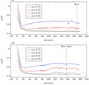
145
discussed adaptation of the PSO algorithm to the discrete problem the sum ofX(t)andV(t)may
146
have values in[−vmax,vmax+1], whereas feasible solutions can be only valid permutation matrices
147
satisfying (??), i.e. having exactly one 1 in each row and column.
148
In formula (??) we introduced a functionSxthat is responsible for convertingX(t) +V(t)into a
149
permutation matrix. Speaking strictly,Sxis rather a procedure, as it incorporates some random choices.
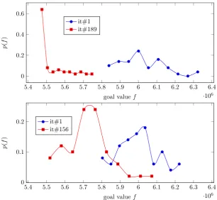
150
In our experiments three variants ofSxprocedures were used:
151
1. Global Max(X)– inniterations, wherenis the size ofX, determines the pivot rowrmand column
152
cm, such that elementxrmcmis the maximal element in unvisited part of the matrixX, than sets 153
xrmcmto 1 and clears other elements in the rowrmandcm[?]. 154
2. PickColumn(X)– picks randomly a pivot columncfromX, than finds a maximum elementxrmc 155
in the columnc, replaces it by 1 and clears other elements in rowrmand columnc.
156
3. SecondTarget(X,Z,d)– similar toGlobal Max(X), however during the firstditerations elements
157
xij, such thatzij =1 are ignored (as the parameterZthe solutionXfrom the last iteration is used
158
(see Algorithm??).
159
TheSecondTarget(X,Z,d)procedure was introduced to avoid undesired behavior, which can be
160
sometimes observed forGlobal Max(X)[?]. In spite of the fact, that particles have velocities far from
161
zero, often they got stuck. We we will discuss this effect on a small 3×3 example. Let us consider the
162
following values of particle state componentsX(t)andV(t).
163
X(t) =
1 0 0 0 0 1 0 1 0
V(t) =
7 1 3 0 4 5 2 3 2
164
Calculation of matrixX(t) +V(t)and than application ofGlobal Maxyields the matrixX(t+1),
165
which is equal to previous positionX(t).
166
X(t) +V(t) =
8 1 3 0 4 6 2 4 2
Sx(X(t) +V(t)) =
1 0 0 0 0 1 0 1 0
167
In such situation, due to the deterministic character ofGlobal Max, the solutionX(t)remains
168
unchanged for several iterations, until another particle reaches a new global minimum, what in
169
consequence modifies(PG(t)−X(t)))component of formula (??) for velocity calculation.
170
This problem can be resolved by altering the order in which pivot elements are chosen in
171
consecutive iterations. An example isPickColumnprocedure, which is more robust, as it introduces
172
some randomness while drawing columns.SecondTargetalgorithm follows another idea: it excludes
173
form the selection process first high rankedd<nelements that in the previous solutionX(t)were
174
already set to 1. Hence, ifdvalue is large enough, it directs to a second solution close toX(t) +V(t).
Let us denote byXdVa pair(X+V,P)whereP=SecondTarget(X+V,X,d). Possible values ofXdV, whered=1 andd=2, are shown below. Elements of a new solutionPare marked with circles, whereas the upper index indicates the iteration, in which the element was chosen.
X1V=
8
2 1 3
0 4 61 2 43 2
X2V=
8 1 32 0
3 4 6
2 41 2
orX2V=
8 1 32 0 41 6 2
3 4 2
It can be observed that for d = 1 the value is exactly the same, as it would result from
176
the Global Max, however setting d = 2 allows to reach a different solution. The pseudocode of
177
SecondTargetprocedure is listed in Algorithm??.
178
Algorithm 1Aggregation procedureSecondTarget Require: X=Z+V- new solution requiring normalization Require: Z- previous solution
Require: depth- number of iterations, in which during selection of maximum element the algorithm ignore
positions, where corresponding element ofZis equal to 1 1: procedureSECONDTARGET(X,Z,depth)
2: R← {1, . . . ,n} 3: C← {1, . . . ,n} 4: foriin (1,n)do
5: CalculateM, the set of maximum elements 6: ifi≤depththen
7: Ignore elementsxijsuch thatzij=1
8: M← {(r,c):zrc6=1∧ ∀i∈R,j∈C,zij6=1(xrc≥xij)}
9: else
10: M← {(r,c):∀i∈R,j∈C(xrc≥xij)} 11: end if
12: Randomly select(r,c)fromM
13: R←R\ {r} .Update the setsRandC
14: C←C\ {c} 15: foriin(1,n)do
16: xri←0 .Clearr-th row
17: xic←0 .Clearc-th column
18: end for
19: xrc←1 .Assign 1 to the maximum element
20: end for 21: returnX 22: end procedure
3.2. Migration
179
The intended goal of the migration mechanism is to improve the algorithm exploration capabilities
180
by exchanging information between swarms. Actually, it is not a true migration, as particles do not
181
move. Instead we modify storedPG[k]solutions (global best solution for ak-th swarm) replacing it by
182
randomly picked solution from a swarm that performed better (see Algortithm??).
183
The newly setPG[k]value influences the velocity vector for all particles ink-th swarm according
184
to the formula (??). It may happen that the goal function value corresponding to the assigned solution
185
PG[k])is worse than the previous one. It is accepted, as the migration is primarily designed to increase
186
diversity within swarms.
Algorithm 2Migration procedure
Require: d- migration depth satisfyingd<m/2, wheremis the number of swarms Require: PG- table of best solutions formswarms
Require: X- set of all solutions 1: procedureMIGRATION(d,PG,X)
2: Sort swarms according to theirPkGvalues into a sequence(s1,s2. . . ,sm−2,sm−1) 3: forkin (1,d)do
4: Randomly choose a solutionxkjbelonging to the swarmsk 5: AssignPG[s
m−k−1]←xkj
6: Update the best goal function value for the swarmm−k−1 7: end for
8: end procedure
It should be mentioned that a naive approach consisting in copying bestPGvalues between the
188
swarms would be incorrect. (Consider replacing line 5 of Algorithm??with:PG[sm−k−1]←PG[sk].)
189
In such case during algorithm stagnation spanning over several iterations: in the first iteration the best
190
valuePG[1]would be cloned, in the second two copies would be created, in the third four and so on.
191
Finally, afterkiterations 2kswarms would follow the same direction. In the first group of experiments
192
reported in Section??we used up to 250 swarms. It means that after 8 iterations all swarms would be
193
dominated by a single solution.
194
3.3. OpenCL algorithm implementation
195
The OpenCL [? ?] is a standard of parallel computing for heterogeneous platforms including
196
GPU, multicore CPU, DSP and FPGA. It defines a common language, programming interfaces and
197
hardware abstraction. OpenCL allows to accelerate computations by decomposing them into a set of
198
parallel tasks calledwork items, which are typically scheduled to operate on separate data.
199
A program on the OpenCL platform is a combination of sequential code executed by the CPUhost
200
and parallel procedures calledkernelsexecuted by multicoredevices. Kernels are written in a restricted
201
C language; the restrictions concern keywords, datatypes and available library functions. The OpenCL
202
provides automatic translation of kernels into the instruction set of the target device. The process
203
occurs once, when they are first time loaded, and takes about 500ms.
204
The OpenCL supports 1D, 2D or 3D organization of data (arrays, matrices and volumes). Hence,
205
data items can be addressed by 1 to 3 indexes and an address within the data range being a single
206
index, a pair or a triple can be used to schedule a kernel instance denoted by the termwork item. To
207
give an example, am×narray of data can be processed in parallel byn·mwork items, which receive
208
at their start a pair of indexes(i,j), 0≤i<mand 0≤j<n. These indexes can be used to select data
209
items assigned to kernels.
210
Work items can be organized intoworkgroups. Within a workgroup, they may share fast local
211
memory and synchronize their activities using alocal barriermechanism. The OpenCL supports three
212
types of memory access: global (that is exchanged between the host and the device), local for a work
213
group and private for a work item. In spite of some advantages offered by the decomposition of
214
processing into workgroups, we decided not use this mechanism due to several platform restrictions
215
limiting the number of work items within a workgroup and amount of accessible memory.
216
The algorithm was implemented in Java language usingaparapiplatform [?], which provides the
217
OpenCL bindings as well as a runtime capable of converting Java bytecodes into the OpenCL kernels.
218
The host part of the program was executed on a Java virtual machine, and the kernel code, originally
219
written in Java, was automatically translated into C code by the aparapi and further processed by the
220
OpenCL for execution on a GPU device.
221
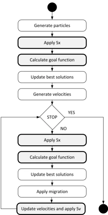
The basic functional blocks of the algorithm are presented in Fig.??. Implemented kernels are
222
marked with gray color. They include particles position update (Apply Sx), velocities update (Update
Generate particles
Apply Sx
Calculate goal function
Update best solutions
Generate velocities
STOP
Apply Sx
Calculate goal function
Update best solutions
Update velocities and apply Sv YES
NO
Apply migration
Figure 1.Functional blocks of OpenCL based algorithm implementation.
velocity and apply Sv) and calculation of the goal function. Other steps are implemented at the host side.
224
This regards also the migration procedure, which sorts swarms indexes in a table according to theirPG
225
value and copies randomly picked entries.
226
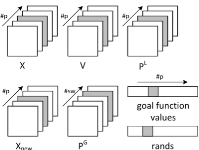
Data ranges selection is an important decision in OpenCL program design. Data used by a particle
227
comprise a number of matrices (see Fig.??):XandXnew– solutions,PL– local best particle solution
228
andV– velocity. They are all stored in large flattened tables shared by all particles. Appropriate table
229
part belonging to a particle can be identified based on theparticle idtransferred to a kernel. Moreover,
230
while updating velocity, the particles reference a tablePGindexed by theswarm id.
231
The memory layout in Fig.??suggests 3D range, whose dimensions are: row, column and particle
232
number. However, the proposed algorithms rather operate on the whole matrices than their parts.
233
Therefore, we decided to use one dimension (particle id) forSxand the goal function calculation, and
234
the two dimensions (particle id, swarm id) for velocity kernels.
235
It should be mentioned that requirements of parallel processing limits applicability of object
236
oriented design at the host side. In particular we avoid creating particles or swarms with their own
237
memory and then copying small chunks between the host and the device. Instead we rather use a
238
flyweight design pattern [?]. If a particle abstraction is needed, a single object can be configured to see
239
parts of large global arraysX,Vas its own memory and perform required operations, e.g. initialization
240
with random values.
#p
X PL
Xnew rands
goal function values
PG
#p
#p #sw
#p
V
#p
Figure 2.Global variables used in the algorithm implementation.
4. Experiments and results
242
In this section we report results of conducted experiments, which aimed at establishing the
243
optimization performance of the implemented algorithm, as well as to collect data related to its
244
statistical properties.
245
4.1. Optimization results
246
The algorithm was tested on several problem instances form the QAPLIB [?], whose size ranged
247
between 12 and 150. Their results are gathered in Table??and Table??. The selection of algorithm
248
configuration parameters (c1,c2andc3factors, as well as the kernels used) was based on previous 249
results published in [? ]. In all cases the second target Sx aggregation kernel was applied (see
250
Algorithm ??), which in previous experiments occurred the most successful.
251
During all tests reported in Table??, apart the last, the total numbers of particles were large:
252
10000-12500. For the last case only 2500 particles were used due to the 1GB memory limit of the GPU
253
device (AMD Radeon HD 6750M card). In this case the consumed GPU memory ranged about 950 MB.
254
The results show that algorithm is capable of finding solutions with goal function values are close
255
to reference numbers listed in the QAPLIB. The gap is between 0% and 6.4% for the biggest casetai150b.
256
We have repeated tests fortai60bproblem to compare the implemented multi-swarm algorithm with
257
the previous single-swarm version published in [?]. Gap values for the best results obtained with the
258
single swarm algorithm were around 7%-8%. For the multi-swarm implementation discussed here the
259
gaps were between 0.64% and 2.03%.
260
The goal of the second group of experiments was to test the algorithm configured to employ
261
large numbers of particles (50 000-100 000) for well knownesc32*problem instances from the QAPLIB.
262
Altough they were considered hard, all of them have been recently solved optimally with exact
263
algorithms [? ?].
264
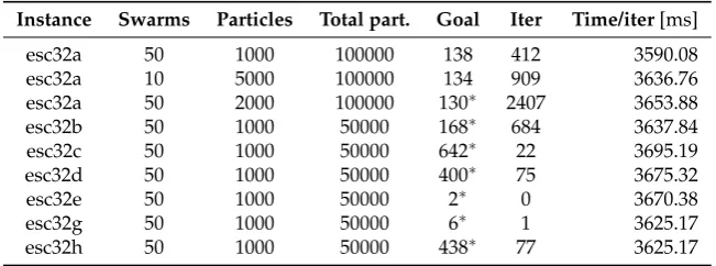
The results are summarized in Table??. We used the following parameters:c1= 0.8,c2 =0.5 265
c3=0.5, velocity kernel: normalized,Sxkernel: second target. During nearly all experiments optimal 266
values of goal functions were reached in one algorithm run. Only the problemesc32aoccurred difficult,
267
therefore for this case the number of particles, as well as the upper iteration limits were increased to
268
reach the optimal solution. What was somehow surprising, in all cases solutions differing from those
269
listed in the QAPLIB were obtained. Unfortunately, our algorithm was not prepared to collect sets of
270
optimal solutions, so we are not able to provide detailed results on their numbers.
271
It can be seen that optimal solutions for problem instancesesc32c–hwere found in relatively small
272
numbers of iterations. In particular, foresc32eandes32g, which are characterized by small values of
273
goal functions, optimal solutions were found during the initialization or in the first iteration.
T able 1. Results of tests for various instance fr om the QAPLIB. No Instance Size
Number of swarms Swarm size Total particles Inertiac1
Table 2.Results of tests foresc32*instances from the QAPLIB (problem sizen=32). Reached optimal values are marked with asterisks.
Instance Swarms Particles Total part. Goal Iter Time/iter[ms]
esc32a 50 1000 100000 138 412 3590.08
esc32a 10 5000 100000 134 909 3636.76
esc32a 50 2000 100000 130∗ 2407 3653.88
esc32b 50 1000 50000 168∗ 684 3637.84
esc32c 50 1000 50000 642∗ 22 3695.19
esc32d 50 1000 50000 400∗ 75 3675.32
esc32e 50 1000 50000 2∗ 0 3670.38
esc32g 50 1000 50000 6∗ 1 3625.17
esc32h 50 1000 50000 438∗ 77 3625.17
The disadvantage of the presented algorithm is that it uses internally matrix representation for
275
solutions and velocities. In consequence the memory consumption is proportional ton2, wherenis
276
the problem size. The same regards the time complexity, which for goal function andSxprocedures
277
can be estimated aso(n3). This makes optimization of large problems time consuming (e.g. even 400 278
sec for one iteration fortai150b). However, for for medium size problem instances, the iteration times
279
are much smaller, in spite of large populations used. For two runs of the algorithmbur26areported
280
in Table??, where during each iteration 12500 particles were processed, the average iteration time
281
was equal 1.73 sec. For 50000-10000 particles and problems of sizen=32 the average iteration time
282
reported in Table??was less than 3.7 seconds.
283
4.2. Statistical results
284
An obvious benefit of massive parallel computations is the capability of processing large
285
populations (see Table ??). Such approach to optimization may resemble a little bit a brutal force
286
attack: the solution space is randomly sampled millions of times to hit the best solution. No doubt that
287
such approach can be more successful if combined with a correctly designed exploration mechanism
288
that directs the random search process towards solutions providing good or near-optimal solutions.
289
In this section we analyze collected statistical data related to the algorithm execution to show that
290
the optimization performance of the algorithm can be attributed not only to large sizes of processed
291
population, but also to the implemented exploration mechanism.
292
The PSO algorithm can be considered a stochastic process controlled by random variablesr2(t) 293
andr3(t)appearing in its state equation (??). Such analysis for continuous problems were conducted 294
in [?]. On the other hand, the observable algorithm outcomes, i.e. the values of goal functions f(xi(t))
295
for solutionsxi,i=1, . . . ,nreached in consecutive time momentst∈ {1, 2, 3, . . .}can be also treated
296
as random variables, whose distributions change over timet. Our intuition is that a correctly designed
297
algorithm should result in a nonstationary stochastic process{f(xi(t)):t ∈ T}, characterized by
298
growing probability that next values of goal functions in the analyzed population are closer to the
299
optimal solution.
300
To demonstrate such behavior of the implemented algorithm we have collected detailed
301
information on goal function values during two optimization task for the problem instancebur26a
302
reported in Table??(cases 2 and 3). For both of them the algorithm was configured to use 250 swarms
303
comprising 50 particles. In the case 2 the migration mechanism was applied and the optimal solution
304
was found in the iteration 156, in the case 3 (without migration) a solution very close to optimal (gap
305
0.06%) was reached in the iteration 189.
306
Fig.??shows values of goal function for two selected particles during run 3. The plots show
307
the typical QAP problem specificity. The PSO algorithm and many other algorithms perform a local
308
neighborhood search. For the QAP problem the neighborhood is characterized by great variations
309
of goal function values. Although mean values of goal function decrease in first twenty or thirty
iterations, the particles behave randomly and nothing indicates that during subsequent iterations
311
smaller values of goal functions would be reached more often.
312
−20 0 20 40 60 80 100 120 140 160 180 200 220 5.4
5.6 5.8 6 6.2
·106
iteration
goal
#4716 #643
Figure 3.Variations of goal function values for two particles exploring the solutions space during the optimization process (bur26a problem instance).
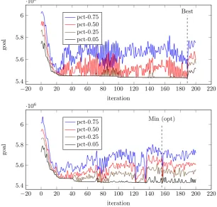
In Fig.??percentile ranks (75%, 50% 25% and 5%) for two swarms, which reached best values in
313
cases 2 and 3 are presented. Although the case 3 is characterized by less frequent changes of scores,
314
than the case 2, probably this effect can not be attributed to the migration applied. It should be
315
mentioned that for a swarm comprising 50 particles, the 0.05 percentile corresponds to just two of
316
them.
317
−20 0 20 40 60 80 100 120 140 160 180 200 220 5.4
5.6 5.8 6
·106
Best
iteration
goal
pct-0.75 pct-0.50 pct-0.25 pct-0.05
−20 0 20 40 60 80 100 120 140 160 180 200 220 5.4
5.6 5.8 6
·106
Min (opt)
iteration
goal
pct-0.75 pct-0.50 pct-0.25 pct-0.05
Figure 4.Two runs of bur26a optimization. Percentile ranks for 50 particles belonging to the most successful swarms: without migration (above) and with migration (below).
Collected percentile rank values for the whole population comprising 12500 particles are presented
318
in Fig.??. For both cases the plots are clearly separated. It can be also observed that solutions very
close to optimal are practically reached between the iterations 20 (37.3 sec) and 40 (72.4 sec). For the
320
whole population the 0.05 percentile represents 625 particles. Starting with the iteration 42 their score
321
varies between 5.449048·106and 5.432361·106, i.e. by about 0.3%.
322
−20 0 20 40 60 80 100 120 140 160 180 200 220 5.4
5.6 5.8 6
·106
Best
iteration
goal
pct-0.75 pct-0.50 pct-0.25 pct-0.05
−20 0 20 40 60 80 100 120 140 160 180 200 220 5.4
5.6 5.8 6
·106
Min (opt)
iteration
goal
pct-0.75 pct-0.50 pct-0.25 pct-0.05
Figure 5.Two runs of bur26a optimization. Percentile ranks for all 12500 particles: without migration (above) and with migration (below).
Fig.??shows, how the probability distribution (the probability mass function - the PMF) changed
323
during the optimization process. In both cases the the optimization process starts with a normal
324
distribution with the mean value about 594500. In the subsequent iterations the maximum of the PMF
325
grows and moves towards smaller values of the goal function. There is no fundamental difference
326
between the two cases, however for the case 3 (with migration) maximal values of the PMF are higher.
327
It can be also observed that in the iteration 30 (completed in 56 seconds) the probability of hitting a
328
good solution is quite high, more then 10%.
329
Interpretation of the PMF for the two most successful swarms that reached best values in the
330
discussed cases is not that obvious. For the case without migration (Fig.??above) there is a clear
331
separation between the initial distribution and the distribution reached in the iteration, which yielded
332
the best result. In the second case (with migration) a number of particles were concentrated around
333
local minima.
334
The presented data shows advantages of optimization performed on massive parallel processing
335
platforms. Due to high number of solutions analyzed simultaneously, the algorithm that does not
336
exploit the problem structure can yield acceptable results in relatively small number of iterations
337
(and time). For a low-end GPU devices, which was used during the test,good enoughresults were
338
obtained after 56 seconds. It should be mentioned that for both presented cases the maximum number
339
of iterations was set to 200. With 12500 particles, the ratio of potentially explored solutions to the
340
whole solution space was equal 200·12500/26!=6.2·10−21.
5.4 5.6 5.8 6 6.2 6.4 ·106
0 5·10−2
0.1 0.15
goal valuef
p
(
f
)
it#1 it#30 it#60 it#120 it#189
5.4 5.6 5.8 6 6.2 6.4 ·106
0 0.1 0.2
goal valuef
p
(
f
)
it#1 it#30 it#50 it#100 it#156
Figure 6.Probability mass functions for 12050 particles organized into 250 x 50 swarms during two runs: without migration (above) and with migration (below).
5.4 5.5 5.6 5.7 5.8 5.9 6 6.1 6.2 6.3 6.4 ·106
0 0.2 0.4 0.6
goal valuef
p
(
f
)
it#1 it#189
5.4 5.5 5.6 5.7 5.8 5.9 6 6.1 6.2 6.3 6.4 ·106
0 0.1 0.2
goal valuef
p
(
f
)
it#1 it#156
5. Conclusions
342
In this paper we describe a multi-swarm PSO algorithm for solving the QAP problem designed
343
for the OpenCL platform. The algorithm is capable of processing in parallel large number of particles
344
organized into several swarms that either run independently or communicate with use of the migration
345
mechanism. Several solutions related to particle state representation and particle movement were
346
inspired by the work of Liu at al. [?], however, they were refined here to provide better performance.
347
We tested the algorithm on several problem instances from the QAPLIB library obtaining good
348
results (small gaps between reached solutions and reference values). However, it seems that for
349
problem instances of large sizes the selected representation of solutions in form of permutation
350
matrices hinders potential benefits of parallel processing.
351
During the experiments the algorithm was configured to process large populations. This allowed
352
us to collect statistical data related to goal function values reached by individual particles. We used
353
them to demonstrate on two cases that although single particles seem to behave chaotically during the
354
optimization process, when the whole population is analyzed, the probability that a particle will select
355
a near-optimal solution grows. This growth is significant for a number of initial iterations, then its
356
speed diminishes and finally reaches zero.
357
Statistical analysis of experimental data collected during optimization process may help to tune
358
the algorithm parameters, as well as to establish realistic limits related to expected improvement of
359
goal functions. This in particular regards practical applications of optimization techniques, in which
360
recurring optimization problems appear, i.e. the problems with similar size, complexity and structure.
361
Such problems can be near-optimally solved in bounded time on massive parallel computation
362
platforms even, if low-end devices are used.
363
References
364
. Koopmans, T.C.; Beckmann, M.J. Assignment problems and the location of economic activities. 365
Econometrica1957,25, 53–76. 366
. Çela, E. The quadratic assignment problem: theory and algorithms; Combinatorial Optimization, Springer: 367
Boston, 1998. 368
. Chmiel, W.; Kadłuczka, P.; Kwiecie ´n, J.; Filipowicz, B. A comparison of nature inspired algorithms for the 369
quadratic assignment problem.Bulletin of the Polish Academy of Sciences Technical Sciences2017,65, 513–523. 370
. Bermudez, R.; Cole, M.H. A Genetic Algorithm Approach to Door Assignments in Breakbulk Terminals. 371
Technical Report MBTC-1102, Mack-Blackwell Transportation Center, University of Arkansas, Fayetteville, 372
Arkansas, 2001. 373
. Mason, A.; Rönnqvist, M. Solution methods for the balancing of jet turbines. Computers & OR1997, 374
24, 153–167. 375
. Grötschel, M. Discrete Mathematics in Manufacturing. ICIAM 1991: Proceedings of the Second 376
International Conference on Industrial and Applied Mathematics; Malley, R.E.O., Ed. SIAM, 1991, pp. 377
119–145. 378
. Sahni, S.; Gonzalez, T. P-Complete Approximation Problems. J. ACM1976,23, 555–565. 379
. Taillard, E.D. Comparison of iterative searches for the quadratic assignment problem. Location Science 380
1995,3, 87 – 105. 381
. Misevicius, A. An implementation of the iterated tabu search algorithm for the quadratic assignment 382
problem.OR Spectrum2012,34, 665–690. 383
. Chmiel, W.; Kadłuczka, P.; Packanik, G. Performance Of Swarm Algorithms For Permutation Problems. 384
Automatyka2009,15, 117–126. 385
. Onwubolu, G.C.; Sharma, A. Particle Swarm Optimization for the assignment of facilities to locations. In 386
New Optimization Techniques in Engineering; Springer, 2004; pp. 567–584. 387
. Liu, H.; Abraham, A.; Zhang, J. A Particle Swarm Approach to Quadratic Assignment Problems. In 388
Soft Computing in Industrial Applications; Saad, A.; Dahal, K.; Sarfraz, M.; Roy, R., Eds.; Springer Berlin 389
. Eberhart, R.; Kennedy, J. A new optimizer using particle swarm theory. Micro Machine and Human 391
Science, 1995. MHS ’95., Proceedings of the Sixth International Symposium on, 1995, pp. 39–43. 392
. Szwed, P.; Chmiel, W.; Kadłuczka, P. OpenCL implementation of PSO algorithm for the Quadratic 393
Assignment Problem. InArtificial Intelligence and Soft Computing; Rutkowski, L.; Korytkowski, M.; Scherer, 394
R.; Tadeusiewicz, R.; Zadeh, L.A.; Zurada, J.M., Eds.; Springer International Publishing, 2015; Vol. Accepted 395
for ICAISC’2015 Conference,Lecture Notes in Computer Science. 396
. Peter Hahn and Miguel Anjos. QAPLIB Home Page. http://anjos.mgi.polymtl.ca/qaplib/. Online: last 397
accessed: Jan 2015. 398
. Fischetti, M.; Monaci, M.; Salvagnin, D. Three Ideas for the Quadratic Assignment Problem.Operations 399
Research2012,60, 954–964. 400
. Anstreicher, K.; Brixius, N.; Goux, J.P.; Linderoth, J. Solving large quadratic assignment problems on 401
computational grids. Mathematical Programming2002,91, 563–588. 402
. Phillips, A.T.; Rosen, J.B. A Quadratic Assignment Formulation of the Molecular Conformation Problem. 403
JOURNAL OF GLOBAL OPTIMIZATION1994,4, 229–241. 404
. Burkard, R.E.; Karisch, S.E.; Rendl, F. QAPLIB - A Quadratic Assignment Problem Library. Journal of Global 405
Optimization1997,10, 391–403. 406
. Hahn, P.M.; Zhu, Y.R.; Guignard, M.; Smith, J.M. Exact solution of emerging quadratic assignment 407
problems. International Transactions in Operational Research2010,17, 525–552. 408
. Hahn, P.; Roth, A.; Saltzman, M.; Guignard, M. Memory-Aware Parallelized RLT3 for solving Quadratic 409
Assignment Problems.Optimization online2013. 410
. Ahuja, R.K.; Orlin, J.B.; Tiwari, A. A greedy genetic algorithm for the quadratic assignment problem. 411
Computers & Operations Research2000,27, 917–934. 412
. Stützle, T.; Dorigo, M. ACO algorithms for the quadratic assignment problem. New ideas in optimization 413
1999, pp. 33–50. 414
. Gambardella, L.M.; Taillard, E.; Dorigo, M. Ant colonies for the quadratic assignment problem. Journal of 415
the operational research society1999, pp. 167–176. 416
. Fon, C.W.; Wong, K.Y. Investigating the performance of bees algorithm in solving quadratic assignment 417
problems. International Journal of Operational Research2010,9, 241–257. 418
. Clerc, M. Discrete particle swarm optimization, illustrated by the traveling salesman problem. InNew 419
optimization techniques in engineering; Springer, 2004; pp. 219–239. 420
. Owens, J.D.; Luebke, D.; Govindaraju, N.; Harris, M.; Krüger, J.; Lefohn, A.E.; Purcell, T.J. A Survey of 421
general-purpose computation on graphics hardware. Computer graphics forum. Wiley Online Library, 422
2007, Vol. 26, pp. 80–113. 423
. Zhou, Y.; Tan, Y. GPU-based parallel particle swarm optimization. Evolutionary Computation, 2009. 424
CEC’09. IEEE Congress on. IEEE, 2009, pp. 1493–1500. 425
. Tsutsui, S.; Fujimoto, N. ACO with Tabu Search on GPUs for Fast Solution of the QAP. InMassively Parallel 426
Evolutionary Computation on GPGPUs; Tsutsui, S.; Collet, P., Eds.; Natural Computing Series, Springer Berlin 427
Heidelberg, 2013; pp. 179–202. 428
. Maitre, O. Genetic Programming on GPGPU Cards Using EASEA. InMassively Parallel Evolutionary 429
Computation on GPGPUs; Tsutsui, S.; Collet, P., Eds.; Natural Computing Series, Springer Berlin Heidelberg, 430
2013; pp. 227–248. 431
. Krüger, F.; Maitre, O.; Jiménez, S.; Baumes, L.A.; Collet, P. Generic Local Search (Memetic) Algorithm on a 432
Single GPGPU Chip. InMassively Parallel Evolutionary Computation on GPGPUs; Tsutsui, S.; Collet, P., Eds.; 433
Natural Computing Series, Springer Berlin Heidelberg, 2013; pp. 63–81. 434
. Bratton, D.; Kennedy, J. Defining a standard for particle swarm optimization. Swarm Intelligence 435
Symposium, 2007. SIS 2007. IEEE. IEEE, 2007, pp. 120–127. 436
. Howes, L.; Munshi, A. The OpenCL Specification.https://www.khronos.org/registry/cl/specs/opencl-2. 437
0.pdf. Online: last accessed: Jan 2015. 438
. Stone, J.E.; Gohara, D.; Shi, G. OpenCL: A parallel programming standard for heterogeneous computing 439
systems.Computing in science & engineering2010,12, 66. 440
. Howes, L.; Munshi, A. Aparapi - AMD. http://developer.amd.com/tools-and-sdks/opencl-zone/ 441
. Gamma, E.; Helm, R.; Johnson, R.; Vlissides, J.Design Patterns: Elements of Reusable Object-Oriented Software; 443
Pearson Education, 1994. 444
. Nyberg, A.; Westerlund, T. A new exact discrete linear reformulation of the quadratic assignment problem. 445
European Journal of Operational Research2012,220, 314–319. 446
. Fern ´ndez-Martínez, J.; Garc ´na Gonzalo, E. The PSO family: deduction, stochastic analysis and comparison. 447