R E S E A R C H
Open Access
Indoor location method of interference
source based on deep learning of spectrum
fingerprint features in Smart Cyber-Physical
systems
Yunfei Chen
*, Taihang Du
*, Chundong Jiang and Shuguang Sun
Abstract
The intensity acquisition and fluctuation of the signal intensity of the interference source caused by the indoor multipath effect are very great, and there is a problem that the best eigenvalue is difficult to choose. A kind of unsupervised machine learning algorithm is proposed, which can independently identify and select the optimal eigenvalue without relying on the prior information. First, the wave signal filtering is reduced and processed by kernelized principle component analysis (KPCA) algorithm. Then, the eigenvalues are selected and the redundant features are eliminated by adaptive parameter adjustment denoising auto-encoder (APADAE) algorithm. Finally, the feature vectors are classified and identified by Softmax algorithm and the classification process are optimized by the particle swarm optimization (PSO) algorithm. Experimental results of the Smart Cyber-Physical systems show that the algorithm can indirectly improve the accuracy of the source location based on improving the classification accuracy.
Keywords:Indoor positioning, Deep learning, Denoising auto-encoder (DAE), Kernelized principle component analysis (KPCA), Smart Cyber-Physical systems, Spectrometer receiver
1 Introduction
Because of the small size, low power, and portability of new communication jammers such as pseudo-base sta-tions, short interference duration, and high randomness of interference area, it is very difficult to supervise them. Interference source is essentially a radio signal transmit-ter. It covers the frequency band of mobile phone and other communication tools with a large signal intensity. Through the right-signing loophole of a mobile phone, it compels it to link with the pseudo-base station, passively receives spam messages, or leaks security information. People’s lives are deeply affected by it, which causes the regulatory authorities to attach great importance to it.
There are few researches on the location of interference sources [1] in indoor environment. At present, fingerprint method [2] is often used to extract fingerprint features of signals in different locations. Indoor radio wave multipath
effect makes the signals fluctuate greatly. How to extract fingerprint features effectively is very important to the lo-cation accuracy. Spectrum research technology for com-munication signal sources is more advanced, but mostly outdoor research, such as satellite, radar, communication base station, and other radiation sources [3] spectrum research. In the field of indoor positioning, fingerprint enhancement is usually achieved by adjusting the access point (AP) mode. The maximum matching method pro-posed by Zhang et al. [4] aimed to select the best AP com-bination to improve the positioning accuracy. The premise of the method is that there are sufficient AP resources in the region. Reference [5] applied principal component analysis (PCA) and used AP with the highest contribution rate to locate. On the basis of it, Liu et al. [6] improved Kalman filter method, improved the accuracy of signal acquisition, and thus improved the overall position-ing performance. Yin et al. [7] proposed to optimize the positioning efficiency according to AP energy consump-tion. On this basis, the water injection model AP * Correspondence:[email protected];[email protected]
School of Artificial Intelligence, Hebei University of Technology, Tianjin 300130, China
optimized deployment method [8] enhanced fingerprint characteristics to improve the overall positioning effi-ciency. It deployed up to seven positioning APs in a small positioning environment. The enhancement of fingerprint features in the above literature mainly improves the effi-ciency of the localization system by increasing the contri-bution rate of AP matching, but none of them can optimize the system with a small number of AP. In the ac-tual location of the interference source, each additional 1 AP will increase the cost and personnel deployment of the amount of labor collected.
In recent years, artificial intelligence [9–13] and ma-chine learning technology [14,15] have been popularized and applied, in which depth learning training test model [16] is more significant and has been widely used in image resolution pattern recognition and other fields. The quality of feature selection determines the generalization performance. The contributions of this paper are as follows:
1) The spectrum characteristics of interference source signal are taken as the research object in the study. 2) A novel unsupervised machine learning algorithm
based on traditional multi-layer denoising auto-encoder (DAE) [17] is proposed to extract AP multi-position spectrum features from the localized coordinate points. It can independently distinguish and select the optimal unlabeled data features without prior information.
3) In the end, the dimension reduction subset of the labeled data is extracted by KPCA [18]. And we explored deep learning model training, testing, and classifying the output data to improve the
positioning accuracy.
The rest of this paper is organized as follows. Section 2 discusses the methods and indoor interference source location system, followed by the selection and extraction of eigenvalues of spectrum signals models in Section 3. The classifier construction, optimization, and training test are discussed in Section 4. Section 5 shows the choice of experimental equipment and the experimental results. Section 6 concludes the paper with summary and future research directions.
2 Indoor interference source location system and pretreatment
2.1 Methods
This study originates from the need of finding illegal radio stations, and pseudo-base stations have become the focus of the regulatory authorities. Radio interfer-ence sources are essentially radio signal transmitters. The shielding effect of radio waves makes it very difficult to locate interference sources in indoor environment. At
present, indoor location is widely applied in location fin-gerprint information matching method.
In recent years, there have been manystudies on finger-print positioning methods in the field of indoor positio-ning.The fingerprint positioning method mainly include two stages: off-line location fingerprint acquisition to es-tablish database and online positioning. The main task of the off-line phase is to establish the location fingerprint information database by detecting the signal intensity of the location area with a radio spectrum analyzer. In the online positioning stage, the detected signal intensity value is directly compared with the fingerprint database in the server through the algorithm, and then, the position coor-dinates of the signal transmitter can be inferred.
2.2 Indoor interference source location system and pretreatment
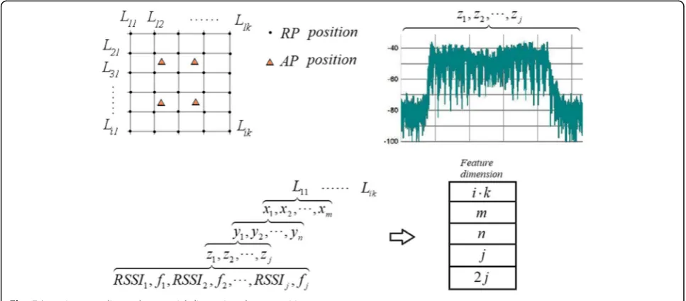
Traditional fingerprint localization methods usually de-ploy multiple AP in the localization area, sample inter-ference sources at a reinter-ference point (RP) location at the same time, and collect all AP received signal strength in-dicators (RSSI) to the server as fingerprint characteris-tics of the point coordinates. There are two difficulties in indoor fingerprint localization of interference sources. First, spectrometer receiver is not suitable for large-scale deployment because of its high price and constrained by the field environment. Second, there are many kinds of interference sources with complex spectrum characteris-tics, and its optimal characteristic parameters are not easy to choose, so it is not suitable to use traditional fin-gerprint method to characterize the location label.
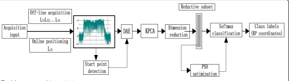
In view of the above problems, this paper proposes a new feature selection localization method. The localization system includes two stages: off-line acquisition and online localization, as shown in Fig.1.
In the off-line acquisition stage, the interference source is deployed in a fixed RP position, and the system only calls an AP to detect the spectrum signal. Test data at multiple differ-ent AP locations around each RP coordinate. That is to say, the spectrum fingerprint features of different points around RP are extracted to represent an RP coordinate of the inter-ference source. In order to build a positioning system, we choose the learning classification strategy training test.
In the online positioning stage, the random position signal samples of the interference source are collected on the spot, and the input system is compared with the database feature space. The coordinates of the interfer-ence source are identified by the classifier according to the RP position class label.
2.3 Off-line acquisition of interference source signal spectrum
and steady-state spectrum characteristics. The former has a short duration and is difficult to capture. There-fore, steady-state spectrum acquisition is the main method in the research.
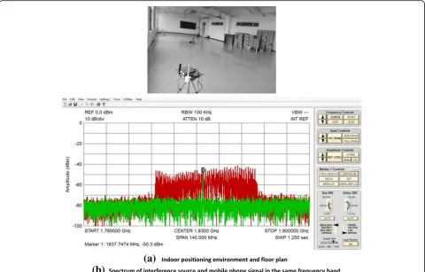
The experimental acquisition is carried out in the 20 m × 13 m open classroom of AI College. The RP coordinates are divided into equal intervals according to the grid. The SA44B spectrum receiver of Signal Corporation of America is deployed on the support of 0.8 m from the center, and the data collected by the receiver is transmitted to the ser-ver through the USB data line. The unlicensed illegal mo-bile phone communication jamming source is deployed on the same level of support of the receiver. Its essence is a modulation signal transmitter with controllable frequency band and mode. It can set up interference modulation mode of CDMA, GSM, DCS, and PHS. Its radio frequency range is 800–1990 MHz, 1 W transmitting power, and 2 dB transmitting antenna gain and can cover radius 30–40 m. The distance between the interference source and the re-ceiver is determined by adjusting the bracket.
The spectrum receiver is set as SignalTrace mode at the system end, which can track the center frequency of the current jammer signal and output the spectrum to the interface. The sampling span SPAN is set to 140 Mhz, and the resolution bandwidth RBW is set to 100 kHz. In order to clearly compare the illegal signal with the normal sig-nal, the jammer is set as DCS mode at the distance of 2 m between AP and RP. Start the detection program to collect the data of the receiver. Sampling time is 1.250 s, and 8561 data points are collected. The interference signals collected separately and the spectrum of the same fre-quency mobile phone dialing signals are superimposed and output to the interface, as shown in Fig.2.
It can be seen from Fig. 2 that the spectrum of the radio signal can be seen:
The mobile phone signal is covered by the high-intensity signal of the interference source, and the spectrum band-width of the interference source is larger than the bandband-width of the mobile phone signal. The peak value of this type of interference source is not unique. Traditional indoor
fingerprint positioning methods mostly collect only one cen-troid frequency and corresponding RSSI values to represent the location characteristics of interference sources in Fig.2. The spectrogram collected by the spectrum analyzer is rough and contains obvious noise, so it is difficult to extract the characteristics of the radio wave signal.
2.4 Interference source signal pre-processing
The rough edge of the signal spectrum will lead to too large error in extracting eigenvalues. By smoothing the noisy sig-nal with the median filter, the sharp edge information can be well preserved. The smoothed spectrum with the median filter still contains noise, which needs to be denoised. In practical applications, the wavelet denoising method has a better effect on the spectrum Gauss white noise suppression. The commonly used wavelet denoising methods include modulus extremum denoising method [19], wavelet correl-ation denoising method [20], and wavelet threshold denois-ing method [21]. The commonly used wavelet threshold algorithms include the hard threshold algorithm and the soft threshold algorithm. However, the hard threshold wavelet denoising algorithm is prone to Gibbs oscillation. And the soft threshold wavelet denoising algorithm is prone to edge distortion due to the constant deviation of wavelet coeffi-cients. A two-stage wavelet threshold function is constructed within the framework of Malat algorithm [22] to balance this problem. The traditional threshold function is improved as follows:
W_ψ;ζ¼ aWψ;ζþð1−aÞsgn Wψ;ζ
Wψ;ζ−bλ;Wψ;ζ≥λ
0;Wψ;ζ<λ
ð1Þ
Among them, the primary threshold is set, and the second-ary threshold is set according to the soft threshold function.
V¼ 1
0:6475 X
δψ ρ ffiffiffiffiffiδ0
p ;
The corresponding adjustment parameters are as follows:
a¼ λ
W0þejλ−δρj; b¼
V−δρ
W0þejV−δρj;
In whichW′is the mean of neighborhood wavelet co-efficients, and the primary threshold corresponds to the
“coarse tuning” signal. The adjustment parametera de-creases with the decrease of the wavelet coefficients in the range of (0, 1). When the wavelet coefficients ap-proach the threshold λ, a→1, when the wavelet coeffi-cients approach zero,a→0, and the wavelet coefficients are updated to δ1¼aρρ after the primary denoising.
The secondary threshold b is independent according to the sparsity of sample points. The adjustment parameter corresponds to the “fine tune” signal, and the wavelet coefficient is updated to δ2=δρ−b∗δρ after secondary
noise reduction. After the two-level threshold thickness is adjusted to denoise the spectrum, the coefficients of each scale operation are used to reconstruct the signal. The API program of the spectrum analyzer is called by LabVIEW software, and combined with MATLAB pro-gramming, the median filter wavelet denoising of inter-ference source input signal is processed, and the
spectrum diagram of noise separation as shown in Fig.3 is obtained.
3 Selection and extraction algorithms of spectrum signal eigenvalues
3.1 Selection of signal characteristics
Traditional eigenvalue extraction mostly adopts manual extraction method, which is inefficient and unsuitable for optimal feature selection. In recent years, deep learn-ing technology has been favored. Among them, DAE algorithm [23] belongs to unsupervised learning algo-rithm. It is based on the application of auto-encoder (AE) [24], which actively distributes unlabeled data into noise, and then trains. The training system acquires noise-free input by learning to remove noise, which is more robust to the training of random input signals. The core of the training system is the extension of the neural network algorithm.
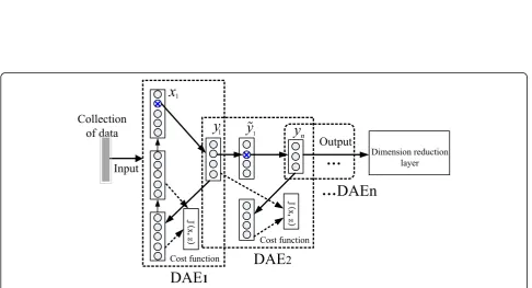
The traditional multi-layer DAE algorithm is modified by artificially setting the number of layers to the adaptive parametric multi-layer embedded APADAE algorithm. As shown in Fig.4, the front DAE1 output layer is linked to the front-end layer of the second DAE2 neuron, and the second DAE2 output is linked to the front-end of
(a)
(b)
Fig. 2Indoor positioning environment and spectrum of interference source and mobile phone signal.aIndoor positioning environment and
(a)
(b)
(c)
Fig. 3Spectrum diagram of filtering and noise reduction processing.aDCS mode interference source signal spectrum.bSignal spectrum after
filtering and denoising.cNoise spectrum component
the back-end neuron. The unlabeled sample data setxis mapped from the DAE1 layer to the hidden layery, and the full connection layer is reconstituted byy toz=g(y) =s(w′y+b′). The minimum value of loss functionL(x,y) constructed byx,y, which is obtained through parameter optimization. Among them,y=s(wx+b),wis the weight matrix of l dimension, w′ is the constraint weight of self-encoder, and it is a reciprocal matrix with w, that is w′=wT, bis deviation function, and sis activation func-tion. The s function is selected as the standard sigmoid function.
In this study, the data in the initial input layer of DAE1 vectorxare“destroyed”by adding artificial noise. The data in x are randomly zeroed proportionally to form~x1 as the input of the next layer of DAE2 and then transmitted to the reconstructed output layer ~z2 via the hidden layer ~y2 of DAE2 mapping. The optimal solution of the system can make the reconstructed error the most by adjusting the parameters of each layer. The cost func-tion is defined as follows:
Jðω;bÞ ¼ arg min1 network and further assumes that the input vector x obeys Bernoulli distribution, so the reconstructed cross-soil loss function is constructed as follows:
Lð~xk;~zkÞ ¼−
Among them, the latter adjusts the weight attenuation and controls the weight of cost function by adjusting the parametera(k−1) to avoid overfitting. Deep learning net-work (DLN) improves the output precision by feedback factor in its back propagation error algorithm. Residual ξ(k)
is defined to represent the difference between recon-structed~yk of DAEklayer network and high-dimensional
input ~zk‐1. The layer k is determined by calculating the minimum loss function iteratively. First, we calculate the residualsξ(k)of the output DAEklayer:
Then, iteratively calculate the residual ξ(k−1) of the hidden layer. From the backpropagation error algorithm,
we can see that the descent vector along the gradient is as follows:
When the above formula converges to the optimum value, the parameter vector ω, b, a(k−1) is used as the optimum adapting parameter of APADAE network model layer and is used to train the sample data. Sample data are input into multi-layer embedded DAE network one by one according to the algorithm flow to select fea-tures and map them to low-dimensional vector output.
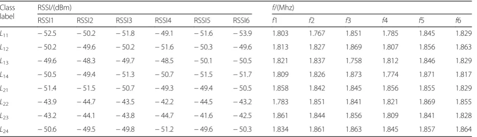
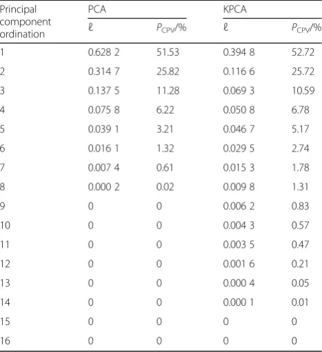
Simplified experiments were conducted to verify the fea-ture selection effect of APADAE algorithm. Six network output nodes were set up, i.e., six feature points selected from the single spectrum. The interference sources were deployed on eight RP coordinates one by one. One AP was fixed at the center of the classroom, and one spectrum was collected by each RP. Each RP label pair was extracted by APADAE algorithm selection. According to the characteristic data of the spectrum map, eight groups of features are extracted. As shown in Table 1, each row corresponds to a class label, each class label cor-responds to six feature points, each feature point corre-sponds to two dimensions (signal strength RSSI and frequencyf), and each feature point corresponds to 12 di-mensions. In the experiment, the parameter vector k of the algorithm APADAE maps to 11 layers of network.
3.2 Analysis of characteristic data
As shown in Table1, it is obvious that unsupervised ma-chine learning method has no prior autonomous feature extraction throughout the spectrum, and its dispersion is high and irregular. As the number of RP labels and AP sampling spectrum increases, its spatial dimension and total feature number will be geometrically doubled.
When the least coordinate labels are collected ass⋅t =8 in the indoor interference source location experi-ment, then m=4 collection points are deployed. Each collection point collectsn=1signal spectrums, and each spectrum selects j=4 feature points. Each feature point corresponds to two parameters RSSI1, f1, RSSI2, f2,
⋯RSSIj, fj, the number is 2j=8. The feature vector set
shows that the overall feature dimension contains m× n×2j=4×3×24=288, and the total quantity is up to m×n×2j×24=288×24=6912Fig.5.
3.3 Dimension reduction
From the analysis of feature data, it can be seen that the increase of data will lead to too much computational complexity, which may lead to“dimension disaster,”and slow data training process will affect generalization abil-ity. Moreover, the feature vectors selected by APADAE algorithm are not all effective, so the redundant feature vectors are eliminated without reducing the classification accuracy, and a feature reduction subset is constructed. The main methods of dimension reduction are com-pressed sensing, principal component analysis, convolu-tion mapping, and threshold filtering.
KPCA is a commonly used nonlinear dimension re-duction method [25]. It is based on the kernel function technique to “kernelize” the linear dimension reduction method. It can be used to improve the ability of princi-pal component analysis (PCA) to analyze nonlinear sam-ple data. Mercer kernel function is introduced into the study, and evaluation parameters are embedded to adjust the proposed method. In order to reduce the dimension of feature data and eliminate the multiple correlations between vectors, the component process is used to ex-tract the high-dimensional nonlinear reduction subset with high cumulative contribution rate.
The feature space data Z= (z1,z2,⋯zj) extracted from
the APADAE algorithm is standardized by ~zi¼ ðzi−μiÞ= σi, μ is the sample mean, and σ is the sample standard deviation, and then, it is mapped to the hyperplane of W= (w1,w2, …,wd).
high-dimensional feature space, so we got the parameter wj. tion is introduced as follows:
κ τi;τj eigenvalue decomposition, the largest eigenvalue ℓ of K and its corresponding eigenvectors are obtained.
νj¼wTjϕ τð Þ ¼
Xm
i¼1
αj
iκ τð i;τÞ ð11Þ
In (11), the j dimension coordinate vector after the mapping of the new data pointτ.
The selection of kernels has great influence on the im-plementation of KPCA. The common kernels are linear kernels, polynomial kernels, Gauss radial basis function, sigmoid kernels, etc. Gauss Radial Basis Kernel (RBF) function is easy to extract local features from different kinds of labels while retaining the overall feature infor-mation. Therefore, it is chosen as a nonlinear relation-ship between the eigenvalues to mine. Its mathematical expression is as follows:
In (12), theεis the radial base nucleus width. In order to measure the interclass separability, we define the hyper parameters dL to adjust the extraction process of
theLprincipal component (class label) process.
Table 1DAE algorithm feature selection simplifies experimental data
dL¼
In (13), we can get dαβis theLprincipal classification
intervals between the α and theβ class label. Then, rLα and rL
β are the maximum distance between theE
princi-pal component and the center of classαand β, respect-ively. And η= |(dα−dβ)|/dLis defined as the adjustment
margin of dL. When η reaches the minimum value, dL
takes the maximum value.
The ratio of extracted principal components to the cu-mulative variance contribution rate of eigenvalues is weighed.
The value of PCPV represents the size of principal component implication information. In order to prevent data from overfitting, we select feature vectors of PCPV value beforecand construct special reduction setsc= 2.
The implementation steps of KPCA dimension reduc-tion algorithm are the following:
Step 1: Initialize the program, normalize the sample data to get the mapping matrix W, and then get the Gauss kernel matrixK;
Step 2: The eigenvalues and eigenvectors are calcu-lated, and the eigenvalues of the correlation coefficient matrix are sorted ℓ1≫ℓ2≫ …≫ℓj, and the eigenvector
v1,v2,…,vjcorresponding to Schmidt orthogonalization
is obtained;
Step 3: ThedLandPCPVare evaluated and evaluated.
Step 4: When η approaches 0.0001, the program ter-minates, and the feature vectors corresponding to the principal components of PCPV before c sort are output to form a new reduced feature set.
3.4 Feature vector extraction
After processing Table 1 data by the KPCA algorithm, where the value of the core width parameter ε is equal to 0.5, we get the eigenvalueℓ and the cumulative con-tribution rate PCPV of the data, and the order is as follows:
Comparing with Table 2, it is obvious that the KPCA algorithm extracts eigenvector components more signifi-cantly than PCA. The PCA algorithm extracts eight vec-tors according to approximate values, while the KPCA algorithm can extract 14 eigenvectors with stronger fea-ture representation ability. The first four of them contain 95.81% of the original signal feature information, but the computational overhead of KPCA algorithm is slightly larger. The feature vectors of the first four ranking values of KPCA algorithm are selected as the feature
representation of the coordinate label, that is, the ori-ginal 16-dimensional feature vectors are replaced by four dimension optimal feature vectors, and the dimension reduction is 1/4 and the labeled optimal feature set is formed.
4 Classifier construction, optimization, and training test
The reduced subset after KPCA processing is classified and processed. The number of classes is equal to the label number or the number of RP coordinates. There are many commonly used shallow learning classification methods: the BP neural network, the support vector ma-chine (SVM) classification, the Softmax classification [26], and so on. Most of the binary classification methods need to change and combine to form a multi-classification pattern. When the dimension is too large, the increase of the classification level results in the slow process of the algorithm.
4.1 The establishment of classifier
According to the analysis of APADAE network algo-rithm, it is obvious that not only dimensionality reduc-tion but also classificareduc-tion funcreduc-tion can be achieved by controlling the number of nodes in the output layer, but the extraction category is rough and inefficient. Softmax classification model, which is widely used in the field of depth learning, and PSO optimization process are in-troduced to improve classification efficiency. The core of this research is to normalize the mapping values of
Table 2The data of two PCA methods
neurons in the classification layer into class label prob-abilities, which is essentially an extension of the logistic regression model in multi-classification applications.
Defining the feature subset U is {u(1),u(2),⋯u(l)}, l∈[1,L], the probability of input samples according to corresponding class labels is p(L(l)=L|u(l);θ) and to realize Softmax-based multi-class classification, its loga-rithmic regression loss function is defined as:
hθ uð Þl
In the above formula, Lis the number of class labels, and system parameter θ determines the probability of class labels and here assigns θ¼ ðθT1;θT2;⋯θTlÞ. Matrix θ corresponds to the probability of one class label per row. The maximum probability p(L(l)=L|u(l);θ) is the classification label of class u(l)corresponding to l class, and the update cost function is
Qð Þ ¼θ −1
The gradient derivative method is applied to solve the partial derivatives of the classification labels, and the corresponding class label parameter θL is obtained by
the following formula.
4.2 PSO optimizes the classification process
As an evolutionary parallel algorithm, PSO algorithm [27] is widely used because its particles traverse the space iteratively from random solutions and have high precision and fast convergence. PSO is used to optimize the classification model of Softmax in order to speed up the classification process. The steps are as follows:
Step 1: Constructing the cost function of Softmax multi-classification model.
Step 2: The location of particles is initialized in the vector space, where the initial dimension of the particle is 16 and the number of iterations is 100.
Step 3: The fitness functionQ(θ) is adjusted by gradient descent method, and the parameterθLof fitness is verified byK-fold cross-validation. The fold is set to 5. The fitness valueQ(θl) is iteratively calculated
to update the position of particles to achieve global optimization.
Step 4: When the threshold condition is reached, the optimal parameterθLof Softmax can be obtained by outputting the position parameters of the particles. Step 5: In order to prevent the problem of “gradient cliff”in convex optimization processing, the Polyak averaging algorithm is applied to process the output of θLbyq= 100 iterations to getθ
the label corresponding to the probability of sample classification is obtained.
4.3 Training test validation
According to the above strategy of the off-line phase, 8, 12, 16, and 24 RP coordinates were selected respectively as the experimental environment organized in section 1.1, and a spectrum analyzer was collected successively around RP points on four different AP coordinates. Each RP coordinate in DCS mode of interference source sam-pled three groups of spectrum separately. In order to prevent the instantaneous overshoot phenomenon of ac-quisition signal from lasting for 20 s, the acac-quisition time interval was 10 s to extract the steady-state spectrum. The total number of 24, 36, 48, and 72 groups of spectrum were collected respectively. In order to prevent data overtraining, 1/6 of the collected data was randomly selected for classifier training and parameter optimization. The remaining data was used for classifier testing. The performance of classification testing was measured by precision (Pr), recall rate (Rr), and F1 score
In (18), the four parameters TP, TN, FP, and FN cor-respond to the true rate, the true negative rate, the false positive rate, and the false negative rate of the resolution results, respectively.
5 Results and discussion
sources one by one from the edge of the classroom by a single receiving AP according to the grid. The width of the mesh is 0.8 m and 1.2 m, respectively. The AP mov-ing position coordinates are as follows: (2.5, 1.2), (4.5, 1.2), (6.5, 1.2) et al., and the RP position is (2, 1.2), (4, 1.2, 6, 1.2) and so on. In addition, we changed the num-ber of RPs at the same acquisition interval. This makes the dimension of data computation increase from 32 to 288. The experiment is to verify the correlation between dimension and positioning accuracy by changing dimen-sion parameters. We delete the location coordinate data which are far away or unsuitable for acquisition and classify and evaluate them using the method of Softmax (Fig.5). In addition, we compare it with the literature BP [29] and SVM [30] in Table3.
From Table3, it can be seen that when the number of RP is 8, and the grid of RP the location interval distance is selected as one eighth of the width of the test class-room, that the grid of RP is about 1.625 m. When the number parameter of RP increases to the maximum of 24, the interval distance is equal to 24 equal parts of the width of the test room, which is approximately 0.541 m. When RP equals 8, we can get three evaluation values of Pr, Rr, and Fs, which correspond to three algorithms of
BP, SVM, and Softmax. Comparatively speaking, BP al-gorithm obtains higher PR value because of its higher computational complexity than SVM algorithm. The highest PR value of Softmax algorithm is80.2. It can be seen that the training scores of the three classification methods are better in Softmax, followed by BP, and SVM needs to cooperate with a multi-classification strat-egy to make its score the lowest. Obviously, the more to add the number of RP, the higher to get the perform-ance. Considering the limitation of the experimental
environment and the operation cost, the RP selection 16 is relatively optimal.
In the further experiment, RP is equal to 16 and the first three of all classifiers are selected. The interference sources are randomly placed in 32 non-label locations in the room to observe the relationship between resolution accuracy and location error. Five groups of spectrum are detected at each location. The classification results of Softmax and the classification errors of three algorithms are listed in Fig. 6 and Table 4 in terms of space relationship.
It is very obvious that the data in Fig.6 are regular. It is a comparison result of position labels, in which the horizontal and vertical coordinates are from L11 to L44. This is the data collected when the RP parameter is se-lected as 16, which the grid of RP is about 0.813 m. The values of each row and column correspond to the actual position coordinates of the test classroom environment. We can clearly see that the diagonal data is the max-imum probability of locating. For example, we get 91.6 values at L11, and 5.8 and 2.6 values at L12 and L14, re-spectively. This means that when the reference point is selected at L11, about 5 of the 100 measurements are positioned atL12and 2 atL14. Obviously, this is the posi-tioning error. We use the algorithm to express the
Fig. 5Location coordinate data spatial dimension decomposition map
Table 3RP number and feature classification performance
RP number
BP SVM Softmax
Pr Rr Fs Pr Rr Fs Pr Rr Fs
8 73.8 66.2 69.7 63.1 58.8 60.8 80.2 63.6 70.9
12 76.7 65.7 70.7 65.8 61.3 63.4 83.4 65.7 73.5
16 78.3 60.5 68.2 72.6 65.7 68.9 91.1 89.8 90.4
positioning error clearly by comparing the probability. In a word, the data of other coordinates are the same, and the complete positioning error data of the test envir-onment can be obtained through Fig.6.
As can be seen from the test results of mixed matrix and Table4 in Fig.6, there are 16 diagonal matrices for correct classification. The overall correct average recog-nition rate can reach 91.5%, and the overall average posi-tioning accuracy can reach 1.16 m. Softmax classification is more effective than other classifiers in identifying the RP position of interference sources. The recognition rate and positioning accuracy are basically positively corre-lated. At the same time, it is also observed that in the middle area of the location environment, the identifica-tion rate is high, up to 95.2%. And the resoluidentifica-tion errors mostly occur in the corner coordinates of the room, where the signal refraction causes great fluctuation, which confirms that indoor environment has a greater impact on location.
6 Conclusion
By changing the traditional fingerprint positioning method of interference source, a new positioning sys-tem is established, which verifies the positioning ac-curacy and reliability of the new indoor positioning method of interference source. The method of extracting spectrum characteristic parameters of in-door interference sources is effective. The average recognition rate of feature can reach 91.5%, and the average positioning accuracy is 1.16 m, which com-pared with the previous positioning methods is greatly improved. As to the positioning environment in the experiment, the number of samples collected is not positively related to the positioning accuracy, and the 192 dimension of the overall dimension is close to the optimal.
The experimental model in this study can provide a new reference for the realization of indoor jamming source location. When the types of jamming sources and ranging and jamming communication modes are changed, their signal characteristics will change ac-cordingly. This requires a large number of real-time updates of sample data to enrich the location diction-ary. In subsequent experiments and studies, it will be gradually improved.
Fig. 6Feature vector classification results
Table 4Positioning error
BP SVM Softmax
Average error/m 1.41 1.23 1.16
Abbreviations
APADAE:Adaptive parameter adjustment denoising auto-encoder algorithm; DAE: Deep learning, denoising auto encoder; KPCA: Kernelized principle component analysis; PSO: The particle swarm optimization algorithm; SVM: The support vector machine
Acknowledgements Not applicable.
Funding
This paper is supported by the National Natural Science Foundation of China (F2014202264) and the Cooperation Fund of Ministry of industry and information technology (12-MC-KY-14).
Availability of data and materials
Data sharing not applicable to this article as the data ownership attributable to Radio Monitoring Committee of Beijing.
Authors’contributions
YC carried out the spectrum studies and participated in drafting the manuscript. TD conceived of the study, participated in its design and coordination, and reviewed the work. CJ carried out the design of the algorithms and participated in the indoor location experiments. SS participated in the design of the study and performed the data analysis. All authors read and approved the final manuscript.
Competing interests
The authors declare that they have no competing interests.
Publisher’s Note
Springer Nature remains neutral with regard to jurisdictional claims in published maps and institutional affiliations.
Received: 16 November 2018 Accepted: 29 January 2019
References
1. X. Li, E. Björnson, E.G. Larsson, S. Zhou, W. Jing, Massive mimo with multi-cell mmse processing: exploiting all pilots for interference suppression.
EURASIP J. Wireless Commun. Netw.2017(1), 117 (2017)
2. Z. DENG, Y. YU, X. YUAN, N. WAN, L. YANG, Situation and development
tendency of indoor positioning. China Commun.10(3), 42–55 (2013)
3. G.H. Huff, J. Feng, S. Zhang, J.T. Bernhard, A novel radiation pattern and frequency reconfigurable single turn square spiral microstrip antenna. IEEE Microw. Wireless Compon. Lett.13(2), 57–59 (2015)
4. M.H. Zhang, Received-signal-strength-based indoor location in wireless
LANs. Comput. Sci.34(6), 68–71 (2007)
5. H. Guo, N. Reisi, W. Jiang, W. Luo, Soft combination for cooperative
spectrum sensing in fading channels. IEEE Access5, 975–986 (2017)
6. L. Mingxin, S. Jianli, Design and implementation of WLAN indoor
positioning systemmodel based on energy efficiency. Chin. J. Sci. Instrum.
5(35), 1169–1178 (2014)
7. M. Yin, J. Gao, Z. Lin, Laplacian regularized low-rank representation and its applications. IEEE Trans. Pattern Anal. Mach. Intell.38(3), 504–517 (2016)
8. M. Wu, Y. Wu, L. Xiao, M. Ming, A. Liu, Z. Ming, Learning-based synchronous
approach from forwarding nodes to reduce the delay for industrial internet
of things. EURASIP J. Wireless Commun. Netw.2018(1), 10 (2018)
9. V. Sharma, M. Bennis, R. Kumar, Uav-assisted heterogeneous networks for
capacity enhancement. IEEE Commun. Lett.20(6), 1207–1210 (2016)
10. R. Zhu, M. Ma, L. Liu, S. Mao, Cooperative and intelligent sensing: a special section in IEEE access. IEEE Access5, 27824–27826 (2017)
11. A. Boulch, P. Trouvé, E. Koeniguer, F. Janez, B. Le Saux,Learning speckle suppression in SAR images without ground truth: application to sentinel-1 time-series, Geoscience and Remote Sensing Symposium IGARSS 2018–2018 IEEE International (2018), pp. 2366–2369
12. A.Z. Papafragkakis, A.D. Panagopoulos,Impulse radio ultra wideband for
broadband indoor machine-to-machine communication networks: system performance evaluation[C]// international workshop on antenna technology: small antennas, innovative structures, and applications. IEEE(2017) 13. J. Wang, R. Zhu, S. Liu, A differentially private unscented Kalman filter for
streaming data in IoT. IEEE Access6, 6487–6495 (2018)
14. C. Bin, Z. Xi’an, A hybrid indoor positioning method based on propagation
model and lacation fingerprint. Bull. Surveying Mapp.6, 35–38 (2015)
15. Y. Jia, J. Ma, L. Gan, Combined optimization of feature reduction and
classification for radiometric identification. IEEE Signal Process. Lett.24(5), 584–588 (2017)
16. C. Xu, K. Li, Cooperative test scheduling of 3d noc under multiple
constraints based on the particle swarm optimization algorithm. Chin. J. Sci. Instrum.38(3), 765–772 (2017)
17. Y. He, W. Meng, L. Ma, et al.,Rapid deployment of APs in WLAN indoor
positioning system[C]//International ICST Conference on Communications and NETWORKING in China. IEEE Comput. Soc(2011), pp. 268–273
18. I. Dey, P.S. Rossi, Probability of outage due to self-interference in indoor wireless environments. IEEE Commun. Lett.21(1), 8–11 (2017) 19. H. Liu, C. Zhao, L. Xuan, et al., Study on a neural network optimization
algorithm based on improved genetic algorithm. Chin. J. Sci. Instrum.7, 1573–1580 (2016)
20. V.E. Kosmidou, P.C. Petrantonakis, L.J. Hadjileontiadis, Enhanced sign
language recognition using weighted intrinsic-mode entropy and signer’s
level of deafness. IEEE Trans. Syst. Man Cybern. B Cybern.41(6), 1531 (2011)
21. X. Liu, R. Zhu, B. Jalaian, Y. Sun, Dynamic spectrum access algorithm
based on game theory in cognitive radio networks. ACM MONET20(6),
817–827 (2015)
22. Z. Huang, G. Shan, J. Cheng, J. Sun, TRec: an efficient recommendation
system for hunting passengers with deep neural networks. Neural Comput. & Applic. (2018).https://doi.org/10.1007/s00521-018-3728-2
23. M.J. Ho, S.M. Berber, K.W. Sowerby, Indoor cognitive radio operation within
the broadcast tv protection contour. Phys. Commun.23, 43–55 (2017) 24. W. Liu, G. Liu, X. Ji, J. Zhai, Y. Dai, Sound texture generative model guided
by a lossless Mel-frequency convolutional neural network. Access IEEE6, 48030–48041 (2018)
25. F. Gontier, M. Lagrange, P. Aumond, A. Can, C. Lavandier, An efficient audio
coding scheme for quantitative and qualitative large scale acoustic
monitoring using the sensor grid approach. Sensors17, 2758 (2017)
26. Gu, J., Wang, Z., Kuen, J., Ma, L., Shahroudy, A., Shuai, B., Liu,T., Wang, X., Wang, G., Recent advances in convolutionalneural networks. arXiv:1512. 07108 (2015)
27. H. Nam, M. Choi, S. Han, C. Kim, S. Choi, D. Hong, A new filter-bank
multicarrier system with two prototype filters for QAM symbols transmission and reception. IEEE Trans. Wirel. Commun.15(9), 5998–6009 (2016) 28. C. Jiang, H. Zhang, Y. Ren, Z. Han, K.-C. Chen, L. Hanzo, Machine learning
paradigms for next-generation wireless networks. IEEE Wirel. Commun.
24(2), 98–105 (Apr. 2017)
29. O. Steven Eyobu, D. Han, Feature representation and data augmentation for
human activity classification based on wearable IMU sensor data using a
deep LSTM neural network. Sensors18, 2892 (2018)