Large scale risk prediction applied to Genetic Analysis Workshop 17 mini exome sequence data

P R O C E E D I N G S

Open Access

Large-scale risk prediction applied to Genetic

Analysis Workshop 17 mini-exome sequence data

Gengxin Li

, John Ferguson

, Wei Zheng

, Joon Sang Lee

, Xianghua Zhang

, Lun Li

, Jia Kang

, Xiting Yan

,

Hongyu Zhao

From

Genetic Analysis Workshop 17

Boston, MA, USA. 13-16 October 2010

Abstract

We consider the application of Efron’s empirical Bayes classification method to risk prediction in a genome-wide association study using the Genetic Analysis Workshop 17 (GAW17) data. A major advantage of using this method is that the effect size distribution for the set of possible features is empirically estimated and that all subsequent parameter estimation and risk prediction is guided by this distribution. Here, we generalize Efron’s method to allow for some of the peculiarities of the GAW17 data. In particular, we introduce two ways to extend Efron’s model: a weighted empirical Bayes model and a joint covariance model that allows the model to properly incorporate the annotation information of single-nucleotide polymorphisms (SNPs). In the course of our analysis, we examine several aspects of the possible simulation model, including the identity of the most important genes, the differing effects of synonymous and nonsynonymous SNPs, and the relative roles of covariates and genes in conferring disease risk. Finally, we compare the three methods to each other and to other classifiers (random forest and neural network).

Background

The development of disease-risk prediction models based on genome-wide association data is a great chal-lenge to statisticians. A major contributing factor to this difficulty is that the observed effects of the most signifi-cant features in any particular model are likely to be overestimates of their true effects [1]. Because of the complexities of a Bayesian analysis with hundreds of thousands of features, most of the shrinkage techniques that have been proposed to deal with this problem have a frequentist flavor, such as the LASSO (least absolute shrinkage and selection operator) and ridge regression [2]. Although these procedures tend to be computation-ally convenient, the resulting shrinkage could be consid-ered ad hoc compared with an empirical Bayes alternative [3], because for the empirical Bayes alterna-tive model shrinkage is guided directly by both the

proportion of associated variants and the effect sizes for this subset of associated variants.

Genetic Analysis Workshop 17 (GAW17) provided a large-scale mini-exome sequence data set with a high proportion of rare variants. In this data set the number of genes far exceeds the number of samples, and, as a result, finding a good risk prediction model is a difficult chal-lenge. Here, we demonstrate the use of an empirical Bayes algorithm, originally proposed by Efron [4] in a microarray case-control context, that is particular suita-ble to this large-scale data setup. This algorithm is a modified version of linear discriminant analysis (LDA) in which certain parameters, which represent standardized differences in the mean expression for case and control subjects, are shrunk before they are substituted into the LDA rule. In addition to describing some of the subtleties that need to be considered when applying Efron’s method to the GAW17 data (or other genome-wide association data), we develop two extensions that allow us to incor-porate single-nucleotide polymorphism (SNP) annotation information into the prediction rule: the weighted empirical Bayes (WEB) model and the joint covariance

* Correspondence: [email protected] 1

Department of Epidemiology and Public Health, Yale University, 60 College Street, New Haven, CT 06520, USA

Full list of author information is available at the end of the article

(JC) model. To show the competitive performance of our proposed methods, we compare them with other classi-fiers: the random forest and the neural network.

Methods

Choice of gene score

A gene score is a composite value calculated by combining all SNP information within the same gene. Several

advan-tages are gained by applying Efron’s empirical Bayes

method to such gene scores instead of to individual SNPs. First, by pooling SNPs together in the correct way, we can potentially enrich the signal-to-noise ratio of the data. Sec-ond, the dimensionality of the feature space is greatly reduced (from 24,487 SNPs to 3,205 gene scores). Finally, even though LDA as a technique does not require the fea-ture variables to be normal, it is actually an optimal proce-dure if they are. Although the number of rare alleles for a particular SNP cannot be considered a normal variable, applying this assumption to the score for genes that have many SNPs may be more reasonable.

Let X_ij denote the Madsen-Browning gene score [5]

that summarizes SNPs in gene i for individualj. This gene score is calculated as:

X

whereG_ljis the number of rare variants for individual

jat SNP l,Kis the number of SNPs within genei, and

p_l is the empirical minor allele frequency (MAF) at

SNP l. In practice, the Madsen-Browning method,

which up-weights SNPs with a lower MAF when calcu-lating gene scores, gives more coherent results on the GAW17 data, and whole gene scores are calculated based on this pooling method.

Method 1: empirical Bayes method

We assume that there are n1 case subjects and n2

con-trol subjects, wherenis the total number of individuals; that is,n=n1 +n2. Suppose that there is no correlation

between different gene scores; then the LDA rule is to classify an individual havingNgene scores (X1, …,XN) as belonging to the disease or case group if:

di i

trol group, and si is the common standard deviation of the interindividual gene score values for geneiin either the case or control group. To apply such a method to real data, all the parameters in Eq. (2) must be esti-mated. Ifsiis known, then theZtest statistic:

Z_i c Xi Xi N

has expectationδ_iand is approximately normally dis-tributed. A naive application of LDA would assign an individual to the disease group if:

Z Wi i

In practice, one would want to consider only genes with the largest Z statistics in application of Eq. (2), effectively restricting the range of the sum to the subset of the most associated genes. Unfortunately, a large selection bias is associated with using the Z statistics directly for this subset of genes, because they are most likely large overestimates of the true values ofδ_i. How-ever, if we can assume that Z_i is normally distributed with variance 1 (which is true asymptotically no matter what the distribution of the original X_i), we can apply the empirical Bayes approach to obtain a Bayes estimate ofδ_ithat will effectively shrinkZ_itoward zero using an empirically estimated prior distribution. These Bayes estimates of δ_ican then be substituted for Z_iin Eq. (7) to produce a better prediction rule, which assigns an individual to the disease group if:

where S is the subset of genes showing the largest marginal association with the disease.

Model 2: weighted empirical Bayes model

We expected that nonsynonymous SNPs are more likely to be directly involved in disease pathogenesis than synonymous SNPs. In this section, we propose a method to incorporate this annotation information into the empirical Bayes model. By fixing gene i, we separately consider two gene scores calculated by restricting the set of SNPs to contain only synonymous or only

nonsy-nonymous SNPs. We denote these gene scores as X_in

and Xis, respectively. The relative importance of the

nonsynonymous SNPs compared to the synonymous SNPs in geneican be measured as:

w p

gene score from the nonsynonymous SNPs and the

synonymous SNPs, respectively. These p-values were

calculated by fitting a logistic regression model in which the disease trait is regressed on either the synonymous or nonsynonymous gene and the Smoke covariate. A

larger wi implies that the nonsynonymous SNPs from

theith gene have a relatively strong association with the disease trait compared with the synonymous SNPs. Throughout this section, the superscriptsn ands refer to nonsynonymous and synonymous, respectively. The other notation is consistent with that introduced in the Model 1 subsection.

By combining the gene weight with the gene scores from both nonsynonymous SNPs and synonymous SNPs, we create a new gene score (weighted score):

X_i*=w X_{i i}n+ −(1 w X_i) _is fori=1,...,N. (11) In this setting, the LDA rule is to classify an individual with new measurements (X_i*,...,X_N* ) as belonging to the disease group if:

d_{i i}

As before, di* is estimated by shrinking Z*i using the

empirical Bayes method developed by Efron [4]. The test statistic:

still follows a normal distribution with expectation d_i* and variance 1; then the application of LDA would assign an individual in the same way.

Model 3: joint covariance model

The strong linkage disequilibrium (LD) between nonsy-nonymous SNPs and synonsy-nonymous SNPs for any particu-lar gene may induce nonsynonymous SNPs and synonymous SNPs to be highly correlated. This correla-tion may greatly affect the eventual predicting result. Building a bivariate model to incorporate nonsynon-ymous and synonnonsynon-ymous SNP information simulta-neously will properly overcome this difficulty. More realistically, we can assume that:

X X

After some algebra, it follows that the optimal LDA rule is to assign an individual to the disease group if:

WiT i i

different populations of parameters, and, as a result, the associated empirically estimated prior distributions should be different. This motivates shrinking the

nonsy-nonymous and synonsy-nonymous Z values separately and

then applying the resulting Bayes estimates into Eq. (17). If there is evidence in the data that the nonsynon-ymous SNPs are more powerful in distinguishing between disease and nondisease, then the synonymous SNPs will be shrunk more. This implicitly gives the non-synonymous gene scores higher weight in the prediction rule.

Other issues: multiple replicates, treatment of covariates, and cross-validation and selection

genes in specific pathways from the 1000 Genomes Project [6]. A unique feature of the GAW17 data is that a large proportion of rare variants are reliably observed in most of the 200 replicates of the data set. Thus for any particular genei, we can define Z statis-tics forRreplicates {Z_i1,…, ZiR}, each of which has an variance 1. A naive analysis would propose:

Var Z R

i

( )

However, one would expect that:

r =Cor

(

)

because there should be a tendency for the sets of individuals having the disease phenotype for any two different replicates to have significant overlap. Under the assumption that:

r =Cor

(

)

for the sth replicate and tth replicate for the ith gene,

Var Z R

R

i

( )

We can then standardize Zi appropriately as:

Z Z

Because the new variables Z*_i have variance 1, Efron’s

shrinkage algorithm can be applied directly to

Z1*,...,Z3205*

{

}

the Bayes estimates of:

E Z E Z

are then substituted into Eq. (9). To estimate r, we assume the relationship:

The second issue in the models is the treatment of covariates. The covariates available in the GAW17 data (i.e., age, sex, and smoking status) have a dominant role in conferring disease risk, and it does not make sense to shrink these variables. When we allow covariates into our prediction rule, the prediction formula becomes:

d i i   

i S

W +Z W +Z W +Z W >

∈

∑

The last issue we want to mention is cross-validation and selection of the best subset of genes. Cross-validation is necessary to select the number of genes involved in any of the prediction rules to avoid the bias of prediction error. Cross-validation is implemented by using 50 repli-cates of the GAW17 data as training data, 50 replirepli-cates as test data, and the other 100 replicates as validation data. TheZscores and associated Bayes estimates are calculated on the training data. The error is evaluated on the test data using the prediction rule for each possible number of genes until we have clearly found the prediction rule with the minimum cross-validation error. The best prediction rule is finally applied to the validation data to find an unbiased estimate of the cross-validation error. The opti-mal number of genes to use in the prediction rule is calcu-lated based on the prediction accuracy on the test data set. It should be noted that for the cross-validation we use a rule of the form:

di i i N

W c

≤

to account for the imbalance between case and control samples in the actual GAW17 data.

Other classifiers

To evaluate the competitive performance of our pro-posed methods, we also fitted a random forest classi-fier [7] and a neural network classiclassi-fier to the GAW17 data. The random forest classifier is known to perform remarkably well on a large variety of risk prediction problems (see [8]) and has been extensively used in genomic applications. The comparable performance to other classification methods, such as diagonal linear

discriminant analysis (DLDA), K nearest neighbor

(KNN) analysis, and support vector machines (SVM), has been demonstrated in a microarray study [9], and the successful application to a large data set has been demonstrated in a genome-wide association study [10]. The technique works by fitting a large number of clas-sification or regression trees to bootstrapped versions

of the original data set and then averaging over all these trees to form the prediction rule. The neural net-work classifier is another efficient learning method and has been widely used in many fields, especially risk prediction [8].

Results

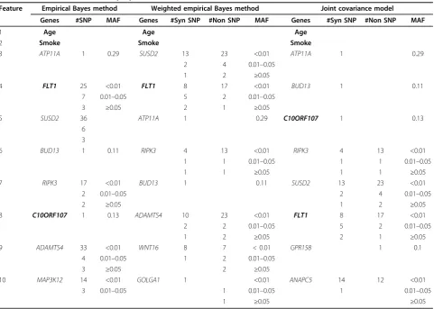
Table 1 displays the 10 most important variables that were found using the empirical Bayes (EB), weighted empirical Bayes (WEB), and joint covariance (JC) methods. It is clear that the environmental variables Age and Smoke have extremely strong signals and dominate the resultant models whenever they are

included. In addition, the gene FLT1 expresses a

strong association with the disease trait and is found in the gene list for these three methods. We also

detected another gene,C10ORF107, that is near to the

true causal gene SIRT1. If we extend the gene list to

the 30 most highly associated genes, PIK3C2B, another

Table 1 Prediction rule of three proposed methods

Feature Empirical Bayes method Weighted empirical Bayes method Joint covariance model

Genes #SNP MAF Genes #Syn SNP #Non SNP MAF Genes #Syn SNP #Non SNP MAF

1 Age Age Age

2 Smoke Smoke Smoke

3 ATP11A 1 0.29 SUSD2 13 23 <0.01 ATP11A 1 0.29

2 4 0.01–0.05

1 2 ≥0.05

4 FLT1 25 <0.01 FLT1 8 17 <0.01 BUD13 1 0.11

7 0.01_–0.05 5 2 0.01_–0.05

3 _≥0.05 2 1 _≥0.05

5 SUSD2 36 ATP11A 1 0.29 C10ORF107 1 0.13

6 3

6 BUD13 1 0.11 RIPK3 4 13 <0.01 RIPK3 4 13 <0.01

1 1 0.01–0.05 1 1 0.01–0.05

1 1 ≥0.05 1 1 ≥0.05

7 RIPK3 17 <0.01 BUD13 1 0.11 SUSD2 13 23 <0.01

2 0.01–0.05 2 4 0.01–0.05

2 ≥0.05 1 2 ≥0.05

8 C10ORF107 1 0.13 ADAMTS4 10 23 <0.01 FLT1 8 17 <0.01

2 2 0.01–0.05 5 2 0.01–0.05

1 2 ≥0.05 2 1 ≥0.05

9 ADAMTS4 33 <0.01 WNT16 8 7 < 0.01 GPR158 1 0.1

4 0.01_–0.05 1 2 0.01_–0.05

3 _≥0.05 2 _≥0.05

10 MAP3K12 14 <0.01 GOLGA1 1 <0.01 ANAPC5 14 12 <0.01

3 0.01–0.05 1 0.01–0.05 1 0.01–0.05

1 ≥0.05 ≥0.05

true causal gene, is involved in the prediction rule. Under the simulation design for the GAW17 data set, if a large proportion of rare variants are involved in this data set, then we need to record the number of SNPs and the minor allele frequency (MAF) interval of SNPs within these highly significant genes (see Table 1). It is obvious that the MAF of most SNPs within these selected genes is less than 0.01. Both the WEB and JC methods incorporate SNP annotation information in the models; the number of SNPs is further divided into two groups: the number of synon-ymous SNPs and the number of nonsynonsynon-ymous SNPs. When compared with the synonymous SNPs, the important genes in Table 1 have a larger propor-tion of nonsynonymous rare variants in the WEB and JC models.

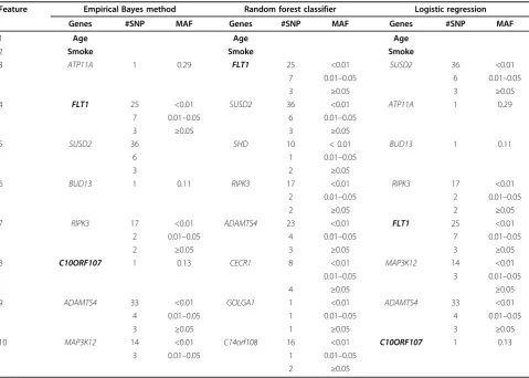
The feature selection procedure of the EB method is also compared with the random forest (RF) method and logistic regression (LR). The comparison results are

summarized in Table 2. According to the RF classifier, 10 features with the largest sum importance score are selected from separate RF classifiers on each of the 100 replicates. Under LR, 10 features with the smallest p -values are chosen from the 100 replicates. In brief, six features in the RF method and 10 features in LR are consistent with features in the EB model, and the con-cordance rate in feature selection is quite high between our proposed methods and other classifiers.

The comparison results of misclassification error for our proposed methods are displayed in Table 3. The first row in Table 3 gives the average misclassification error obtained from the model derived on the training and test data to predict the phenotype values of the 100 validation replicates (see the earlier discussion of cross-validation). Note that this error may depend on which 100 replicates are chosen. To explore this issue, we ran-domly split the 200 replicates into training, test, and validation sets five times. This enabled us to compute a

Table 2 Comparison of the prediction rule between the empirical Bayes and other classifiers

Feature Empirical Bayes method Random forest classifier Logistic regression

Genes #SNP MAF Genes #SNP MAF Genes #SNP MAF

1 Age Age Age

2 Smoke Smoke Smoke

3 ATP11A 1 0.29 FLT1 25 <0.01 SUSD2 36 <0.01

7 0.01–0.05 6 0.01–0.05

3 ≥0.05 3 ≥0.05

4 FLT1 25 <0.01 SUSD2 36 <0.01 ATP11A 1 0.29

7 0.01_–0.05 6 0.01_–0.05

3 _≥0.05 3 _≥0.05

5 SUSD2 36 SHD 10 < 0.01 BUD13 1 0.11

6 1 0.01–0.05

3 2 ≥0.05

6 BUD13 1 0.11 RIPK3 17 <0.01 RIPK3 17 <0.01

2 0.01–0.05 2 0.01–0.05

2 ≥0.05 2 ≥0.05

7 RIPK3 17 <0.01 ADAMTS4 23 <0.01 FLT1 25 <0.01

2 0.01–0.05 4 0.01–0.05 7 0.01–0.05

2 ≥0.05 3 ≥0.05 3 ≥0.05

8 C10ORF107 1 0.13 CECR1 8 <0.01 MAP3K12 14 <0.01

0.01–0.05 3 0.01–0.05

4 ≥0.05 ≥0.05

9 ADAMTS4 33 <0.01 GOLGA1 1 <0.01 ADAMTS4 33 <0.01

4 0.01_–0.05 1 0.01_–0.05 4 0.01_–0.05

3 _≥0.05 1 _≥0.05 3 _≥0.05

10 MAP3K12 14 <0.01 C14orf108 16 <0.01 C10ORF107 1 0.13

3 0.01–0.05 1 0.01–0.05

2 ≥0.05

standard error of the mean prediction error for the EB, WEB, and JC methods (see Table 3). Note that the dif-ferences between the means are large relative to the standard errors and likely reflect true differences in the performance of the three methods. It is clear that the WEB method provides the smallest average misclassifi-cation error (0.236) followed by the JC method (0.241) and the EB method (0.26).

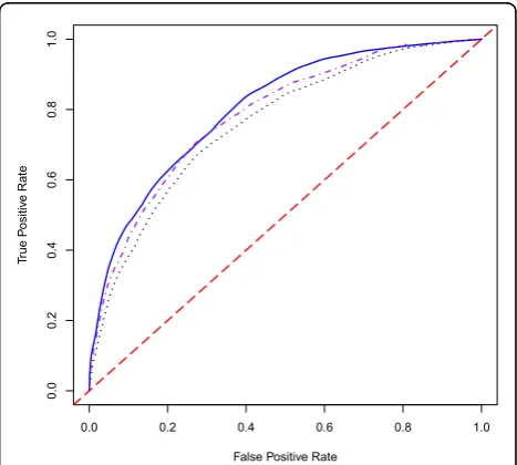
We also compared the prediction accuracies for our proposed methods using the area under curve (AUC) value (Table 3). When both genes and environmental variables are involved in the prediction model, the WEB method gives the highest AUC value (0.80) followed by the JC method (0.78) and the EB method (0.76). All three methods perform better than other classifiers: RF (0.67), neural network 1 (NN1: 0.68), and neural net-work 2 (NN2: 0.70) (Table 4). It is easy to see that the EB-based neural network classifier (0.70) provides a lar-ger AUC value than the LR-based neural network classi-fier (0.68). The relevant three receiver operating characteristic (ROC) curves corresponding to our pro-posed methods are plotted in Figure 1.

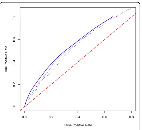
In summary, our proposed methods significantly improve the accuracy of the prediction model com-pared with other classifiers. Because the environmental variables have such a strong influence in the prediction model, we also fitted the EB, WEB, and JC models using the genetic variables alone in order to determine the prediction accuracy achievable through purely genetic information (Table 3). In this case, the best AUC value is achieved using the WEB method (0.64) followed by the JC method (0.62) and the EB method (0.60) (Figure 2).

Of course, in practical applications more than one replicate cannot be obtained. This scenario can be

represented by training and testing the prediction model using only one replicate. When one does this, the prediction model based on the EB method is still quite good. For example, FLT1 is always in the list of the 10 most strongly associated features in the EB model. If a similar model is fitted using the RF classi-fier, no causal genes tend to be found in the top gene list (Table 5). In addition, the EB method provides a Table 4 Comparison of AUC value for the empirical Bayes and other classifiers

Item Model Statistics Empirical Bayes model Random forest classifier Neural network 1 Neural network 2

AUC value Gene + environment Mean 0.76 0.67 0.68 0.70

SE 0.0102 _{– – –}

AUC value indicates the area under the ROC curve when minimizing the cross-validation error. Neural network 1 used selected features from the logistic regression; neural network 2 used selected features from the empirical Bayes method. SE is the standard error of the AUC value.

Table 3 Cross-validation error and AUC value for the three methods

Item Model Statistic Empirical Bayes method Weighted empirical Bayes method Joint covariance model

Cross-validation error Gene + environment Mean 0.26 0.24 0.24

SE 0.0020 0.0011 0.0012

AUC value Gene + environment Mean 0.76 0.80 0.78

SE 0.0102 0.0015 0.0148

AUC value Gene Mean 0.60 0.64 0.62

SE 0.0191 0.0183 0.0191

AUC is the area under the ROC curve when minimizing the cross-validation error. SE, standard error of the cross-validation error and the AUC value.

0.0 0.2 0.4 0.6 0.8 1.0

0.0

0.2

0.4

0.6

0.8

1.0

False Positive Rate

Tr

ue P

ositiv

e Rate

Figure 1ROC curves for the EB, WEB, and JC methods for the prediction model using genes and environmental covariates.

substantively larger AUC value (0.72) than the RF clas-sifier (0.66) (Table 6).

Conclusions

It is well known that developing a good disease risk pre-diction model based on genome-wide association data is a difficult task; the number of predictors can be orders of magnitude higher than the number of samples that are genotyped. This is certainly the case in the GAW17 mini-exome data set, in which there is information on 24,487 SNPs for only 697 samples. In this paper, we have used the good properties of the empirical Bayes prediction model that Efron [4] developed in a large-scale microarray context to build a prediction model for these data. An interesting feature of the GAW17 data is that they provide annotation information for each SNP in the form of a synonymous/nonsynonymous indicator. Because only nonsynonymous SNPs affect protein func-tion, we expect that they, rather than synonymous SNPs, are more likely to be directly involved in disease pathogenesis. We propose two ways (weighted empirical Bayes model and joint covariance model) to properly incorporate this annotation information into the predic-tion model. The weighted empirical Bayes model pro-vides the best performance (relatively small cross-validation error and larger AUC value). We also com-pare the three EB classifiers with two other popular clas-sifiers (random forest and neural network). The EB

Table 5 Prediction rule for two classifiers based on one replicate

Feature Empirical Bayes classifier Random forest classifier

Genes #SNP MAF Genes #SNP MAF

1 Age Age

2 Smoke Smoke

3 GOLGA1 1 <0.01 OR1L6 <0.01

1 0.01–0.05 3 0.01–0.05

1 ≥0.05 1 ≥0.05

4 FLT1 25 <0.01 VTI1B 9 <0.01

7 0.01–0.05 1 0.01–0.05

3 ≥0.05 1 ≥0.05

5 NFKBIA 6 <0.01 DENND1A 19 <0.01

0.01–0.05 3 0.01–0.05

2 ≥0.05 4 ≥0.05

6 DGKZ 17 <0.01 C9ORF66 4 <0.01 4 0.01–0.05 3 0.01–0.05

1 ≥0.05 4 ≥0.05

7 SMTN 23 <0.01 CECR1 8 <0.01

4 0.01–0.05 0.01–0.05

2 ≥0.05 4 ≥0.05

8 PAK7 1 0.30 MAP3K12 14 <0.01

3 0.01–0.05 ≥0.05

9 ADAM15 22 <0.01 SLC20A2 24 <0.01

5 0.01–0.05 4 0.01–0.05

3 ≥0.05 1 ≥0.05

10 ADAMTS4 33 <0.01 ALK 9 <0.01

4 0.01–0.05 1 0.01–0.05

3 ≥0.05 6 ≥0.05

Top 10 important features from the model incorporating genes and environmental variables (Age and Smoke) using one replicate between our proposed method (empirical Bayes) and the random forest method. #SNP, number of SNPs within a specific gene. MAF shows three intervals of minor allele frequency: MAF < 0.01, 0.01≤MAF < 0.05, and MAF > 0.05. The boldfaced gene FLT1 still can be selected in the empirical Bayes method but is not observed using the random forest method.

Table 6 Cross-validation error and AUC value for the empirical Bayes and random forest methods based on one replicate

Item Model Statistics Empirical

Bayes method

Random forest method

Cross-validation error

Gene + environment

Mean 0.26 0.23

SE 0.009 –

AUC value Gene + environment

Mean 0.72 0.66

SE 0.058 –

AUC value is the area under the ROC curve when minimizing the cross-validation error. SE is the standard error of the cross-cross-validation error and the AUC value.

0.0 0.2 0.4 0.6 0.8

0.0

0.2

0.4

0.6

0.8

False Positive Rate

Tr

ue P

ositiv

e Rate

Figure 2ROC curves for the EB, WEB and JC methods for the

prediction model using genes only. The black dotted line is the

classifiers have superior prediction performance in terms of AUC value. Based on this analysis, we think that Efron’s empirical Bayes risk prediction model, extended in the manner that we describe here, is a useful and powerful tool for disease risk prediction in genome-wide association studies.

Acknowledgments

We thank the reviewers and editors for their insightful and constructive comments on our manuscript. We also thank the Yale University Biomedical High Performance Computing Center and the National Institutes of Health (NIH), which funded the instrumentation through grant RR19895. This project is supported in part by NIH grants R01 GM59507 and T15 LM07056 and by a fellowship award from the China Scholarship Council. The Genetic Analysis Workshop 17 is supported by NIH grant R01 GM031575.

This article has been published as part ofBMC ProceedingsVolume 5 Supplement 9, 2011: Genetic Analysis Workshop 17. The full contents of the supplement are available online at http://www.biomedcentral.com/1753-6561/5?issue=S9.

Author details 1

Department of Epidemiology and Public Health, Yale University, 60 College Street, New Haven, CT 06520, USA.2_{Keck Laboratory, Yale University, 300} George Street, New Haven, CT 06511, USA.3_{Department of Electronic} Science and Technology, University of Science and Technology of China, Hefei, China.4_{Bioinformatics and Molecular Imaging Key Laboratory,} Huazhong University of Science and Technology, Wuhan, China.

Authors’contributions

GL carried out the design of models, data analysis, and wrote the draft, JF carried out the design of models and wrote the manuscript, WZ participated in preparing the gene score data and performed random forest analysis, JSL, XZ and LL participated in preparing the gene score data, JK participated in the comparison results between our proposed methods and other classifiers, XY participated in the progression of studies, HZ managed the progression of this project and reviewed the draft. The final manuscript has been approved by all authors after they read it.

Competing interests

The authors declare that there are no competing interests.

Published: 29 November 2011

References

1. Zhong H, Prentice RL:Bias-reduced estimators and confidence intervals for odds ratios in genome-wide association studies.Biostatistics2008,

9:621-634.

2. Tibshirani R:Regression shrinkage and selection via the Lasso.J R Stat Soc B1996,58:267-288.

3. Robert C:The Bayesian Choice.New York, Springer Texts in Statistics;, 2nd 2001.

4. Efron B:Empirical Bayes estimates for large-scale prediction problems.J Am Stat Assoc2009,104:1015-1028.

5. Madsen BE, Browning SR:A groupwise association test for rare mutations using a weighted sum statistic.PLoS Genet2009,5:e1000384, doi:10.1371/ journal.pgen.1000384.

6. Almasy L, Dyer TD, Peralta JM, Kent JW Jr, Charlesworth JC, Curran JE, Blangero J:Genetic Analysis Workshop 17 mini-exome simulation.BMC Proc2011,5(suppl 8):S2.

7. Breiman L: Random forests.Machine Learning2001,45:5-32. 8. Hastie T, Tibshirani R, Friedman J:The Elements of Statistical Learning:

Data Mining, Inference, and Prediction.New York, Springer Series in Statistics;, 2nd 2009.

9. Diaz-Uriarte R, Alvarez de Andres:Gene selection and classification of microarray data using random forest.BMC Bioinformatics2006,7:3.

10. Goldstein BA, Hubbard AE, Cutler A, Barcellos LF:An application of random forests to a genome-wide association data set: methodological considerations and new findings.BMC Genet2010,11:49.

doi:10.1186/1753-6561-5-S9-S46

Cite this article as:Liet al.:Large-scale risk prediction applied to Genetic Analysis Workshop 17 mini-exome sequence data.BMC Proceedings20115(Suppl 9):S46.

Submit your next manuscript to BioMed Central and take full advantage of:

• Convenient online submission

• Thorough peer review

• No space constraints or color figure charges

• Immediate publication on acceptance

• Inclusion in PubMed, CAS, Scopus and Google Scholar

• Research which is freely available for redistribution