Weighted sum rate maximization for multi user SIMO multiple access channels in cognitive radio networks

R E S E A R C H

Open Access

Weighted sum-rate maximization for

multi-user SIMO multiple access channels in

cognitive radio networks

Peter He

, Lian Zhao

and Jianhua Lu

Abstract

In this article, an efficient distributed and parallel algorithm is proposed to maximize the sum-rate and optimize the input distribution policy for the multi-user single input multiple output multiple access channel (MU-SIMO MAC) system with concurrent access within a cognitive radio (CR) network. The single input means that every user has a single antenna and multiple output means that base station(s) has multiple antennas. The main features are: (i) the power distribution for the users is updated by using variable scale factors which effectively and efficiently maximize the objective function at each iteration; (ii) distributed and parallel computation is employed to expedite convergence of the proposed distributed algorithm; and (iii) a novel water-filling with mixed constraints is investigated, and used as a fundamental block of the proposed algorithm. Due to sufficiently exploiting the structure of the proposed model, the proposed algorithm owns fast convergence. Numerical results verify that the proposed algorithm is effective and fast convergent. Using the proposed approach, for the simulated range, the required number of iterations for convergence is two and this number is not sensitive to the increase of the number of users. This feature is quite desirable for large scale systems with dense active users. In addition, it is also worth noting that the proposed algorithm is a monotonic feasible operator to the iteration. Thus, the stop criterion for computation could be easily set up.

Keywords: Channel capacity, Multi-user MIMO (MU-MIMO), Multi-access Channels (MAC), Cognitive Radio (CR), Multiple-antenna, Broadcast systems, Maximum sum-rate, Optimal power distribution, Optimization methods, Water-filling, Algorithm with mixed constraints

1 Introduction

The radio spectrum is a precious resource that demands for efficient utilization as the currently licensed spec-trum is severely underutilized [1]. Cognitive radio (CR) [2-4], which adapts the radios operating characteristics to the real-time conditions, is the key technology that allows flexible, efficient and reliable spectrum utilization in wireless communications. This technology exploits the underutilized licensed spectrum of the primary user(s) (PU) and introduces secondary user(s) (SU) to operate on the spectrum that is either opportunistically being available or concurrently being shared by the PU and the SU. Under this situation and according to the defini-tion of a cognitive (radio) network [5], opportunistically

*Correspondence: [email protected]

1Department of Electrical and Computer Engineering, Ryerson University, Ontario,M5B 2K3, Canada

Full list of author information is available at the end of the article

utilizing the spectrum means that the SUs may fill the spectrum gaps or holes left by the PUs; whereas concur-rently utilizing the spectrum means that the SUs trans-mit over the same spectrum as the PUs, in a way that the interference from the transmitting SUs does not vio-late the quality requirement from the PUs. This article focuses on the latter case. Furthermore, the multiple-input multiple-output (MIMO) technology uses multiple antennas at either the transmitter or the receiver to signif-icantly increase data throughput and link range without additional bandwidth or transmitted power. Thus it plays an important role in wireless communications today. In infrastructure-supported networks, such as the widely used cellular network, base stations are typically shared by a large number of users. Within the scope of this article, it is therefore assumed that the base station under con-sideration is shared by multiple PUs and multiple SUs. In this article, a MIMO-enhanced CR network is considered

to fully ensure the quality of service (QoS) of the PUs as well as to maximize the weighted sum-rate of the SUs. We consider multiple SUs accessing the base station, referred to as a multiple-access channel (MAC).

The weighted sum-rate maximization problem is to compute the “best" achievable rate vector in the capacity region [6-8] by specifying the working point at the bound-ary of the capacity region. This optimality problem is of the Pareto meaning under multi-objective optimization.

For the non-CR cases, the sum-rate maximization prob-lem has been intensively explored for both Gaussian broadcast channel (BC) [9,10] and Gaussian MAC [11]. Typical approaches include iterative water-filling algo-rithms [9,11] and dual-decomposition [10]. The conven-tional water-filling algorithm [12] which is an efficient resource allocation algorithm needs to be used inside each of the iterations as an inner loop operation. In addition, the setup of the well known duality between the Gaussian BC and the sum-power constrained Gaussian dual MAC [13-15] facilities the transform of BC sum-rate problems into its dual MAC problem. As for the weighted sum-rate problem, it is easily seen that as the weighted coeffi-cients all being unity, the weighted sum-rate problem is reduced into a sum-rate optimization problem. Thus, solving the weighted sum-rate problem is more general. However, due to the more complicated problem struc-ture, the conventional water-filling algorithm [12] is not able to compute its solution. For computing the maximum weighted sum-rate for a class of the Gaussian single-input multiple-output (SIMO) BC systems or equivalent dual MAC systems [16], has presented some algorithms using a cyclic coordinate ascent algorithm to provide the max-stability policy.

For the CR cases, besides the individual power con-straints to the SUs, the total interference power from the SUs needs to be included into the constraints of the tar-get problem. Since single-antenna mobile users are quite common and compose a major served group due to the size and cost limitations of mobile terminals, this arti-cle is confined to a single input multiple output multiple access channel (SIMO-MAC) in the CR network. Ear-lier study [17,18] investigated the sum-rate problem and the weighted sum-rate problem in CR-SIMO-MAC cases, respectively. In addition, for the ergodic sum capacity of single input single out (SISO) system [19], studied the maximum (non-weighted) sum-rate problem with a simple form of the objective function.

In this article, by exploiting the structure of the weighted sum-rate optimization problem, we propose an efficient iterative algorithm to compute the optimal input pol-icy and to maximize the weighted sum-rate, via solv-ing a generalized water-fillsolv-ing problem in each of the iterations. The water-filling machinery is experiencing continuous development [12,20-23]. In this article, we

propose a generalized weighted water-filling algorithm (GWWFA) to form a fundamental step (inner loop algo-rithm) for the target problem. In the inner loop, the weighted sum-rate problem is decomposed into a series of generalized water-filling problems. With this decom-position, a decoupled system with each equation of the decoupled system containing only a scalar variable is formed and solved. Any one of the equations is solved by the GWWFA with a finite number of loops. To speed up the computation of the solution to each of the equations, we also specify the intervals the solution belongs to.

For the outer loop of the algorithm, a variable scale fac-tor is applied to update the covariance vecfac-tor of the users. The optimal scale factor is obtained by maximizing the target objective value (i.e., the weighted sum-rate) in the scalar variableβto expedite convergence of the proposed algorithm. In order to achieve this purpose, we deter-mine an optimal scale factor by searching in a range which consists of a few discrete values. As a result, parallel oper-ation can be used to expedite the search and to avoid the requirement of another nested loop. This parallel oper-ation can be distributed to and carried out by multiple processors (for example, four processors).

Compared with earlier study [18], the main difference of our study is that: (i) in [18], the dual-decomposition approach [10] is used. In our study, we apply the itera-tive water-filling algorithm [9] and extend the algorithm to solve the target problem. The advantage of the iterative water-filling algorithm is that it is a monotonic feasible operator to the iteration. That is to say, the proposed algo-rithm generates a sequence composed of feasible points in its iterations. The objective function values, correspond-ing to this point sequence, are monotonically increas-ing. Hence, the stop criterion for computation might be easily set up. However, the regular primal-dual method used in [18] is not a feasible point method; (ii) for the constraints of the target problem, we make the individ-ual power constraints more strict and more reasonable, due to the values of signal powers being assumed to be greater than or equal to zero; (iii) the convergence rate is improved significantly. In the numerical example illus-trated by Figure 1 of [18], the convergence of the weighted sum-rate is obtained after 110 iterations for a system with 3 SUs and 2 PUs. However, with our proposed algo-rithm, we achieve the weighted sum-rate convergence with two iterations with the simulated range (number of SUs up to 110). In addition, even if the PUs and SUs are served by different base stations, it is easy to see that the proposed machinery can be used with some minor modifications.

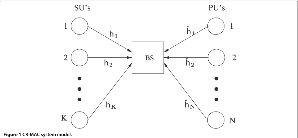
Figure 1CR-MAC system model.

algorithm to solve the maximal weighted sum-rate prob-lem through an inner loop algorithm. The optimality proof of the inner loop algorithm (GWWFA) is presented in Section 3.1. Then the outer loop algorithm (AWCR) and its implementation are presented in Section 3.2. Section 4 provides the convergence proof of the AWCR. Section 5 presents numerical results and some complexity analysis to show the effectiveness of the proposed algorithm.

Key notations that are used in this article are as fol-lows:|A| and Tr(A)give the determinant and the trace of a square matrix A, respectively; E[X] is the expec-tation of the random variable X; the capital symbol I for a matrix denotes the identity matrix with the cor-responding size. A square matrix B 0 means that B is a positive semi-definite matrix. Further, for two arbitrary positive semi-definite matrices B and C, the expression B C means the difference of B − C is a positive semi-definite matrix. In addition, for any complex matrix, its superscripts † and T denote the conjugate transpose and the transpose of the matrix, respectively.

2 SIMO-MAC in CR network and its weighted sum-rate

For a SIMO-MAC in a CR network, as shown in Figure 1, assume that there are one base-station (BS) withNr

anten-nas, andKSUs andNPUs, each of which is equipped with one single antenna. The received signaly ∈CNr×1_{at the}

BS is described as

y =K_j=1h†_jxj+N_j=1hˆ†_jxˆj+z, hj∈C1×Nr, j =1, 2,. . .,K, andhˆj∈C1×Nr,

j =1, 2,. . .,N,

(1)

where thejth entry xj ofx ∈ CK×1 is a scalar complex input signal from the jth SU and xis assumed to be a Gaussian random vector having zero mean with indepen-dent entries. The jth entry xˆj of xˆ is a scalar complex input signal from the jth PU andxˆ is assumed to be a Gaussian random vector having zero mean with indepen-dent entries. The noise term, z ∈ CNr×1_{is an additive}

Gaussian noise random vector, i.e., z ∼ N(0,σ2I). The channel input,xˆ,x, andzare also assumed to be indepen-dent. Furthermore, thejth SU’s transmitted power can be expressed as

Sj=E

|xj|2,j=1, 2,. . .,K. (2) Note thatSj,∀j, is non-negative.

The mathematical model of the weighted sum-rate opti-mization problem for the SIMO-MAC in the CR network can be stated as follows (refer to (2.16) in [6] and the references therein):

Given a group of weights{wk}K_k=1which is assumed to be in decreasing order (users can be arbitrarily renum-bered to satisfy this condition) with the achievable rate of the secondary userk,

log

⎛ ⎝

⎛ ⎝_|C0+

k

j=1

h†_jhjSj|

⎞ ⎠

⎛ ⎝_|C0+

k−1

j=1

h†_jhjSj|

⎞ ⎠ ⎞ ⎠,∀k,

the weighted sum-rate is organized by

fwmac

h†₁,. . .,h†_K;P1,. . .,PK;Pt

=max_{S

k}Kk=1wKlog|C0+

K

j=1h

†

jhjSj|

+ K−1

k=1(wk−wk+1)log|C0+kj=1h

†

jhjSj|

Subject to: 0≤Sk≤Pk,∀k;K_k=1gkSk≤Pt,

where, for the MAC cases, the peak power constraint on the kth SU exists and is denoted by a group of positive numbers:P_k,k=1,. . .,K; the power threshold to ensure the QoS of the PUs is denoted by the positive number Pt. Further, when no confusion is possible,fwmacis simply written asf. For convenience, we defineηkbywk−wk+1 fork = 1,. . .,K −1; andηK bywK, as a group of

non-negative real numbers, and assume at least one of them to be non-zero. Further, the termgk =hkh†k,∀k, is the

chan-nel power gain of thekth SU to the BS. Also, we denote the covariance matrix of the random vectorN_j=1hˆ†_jxˆj+zby C0. It is easy to see that the matrixC0is positive definite.

The constraintK_k=1gkSk≤Ptis called the sum-power

constraint with gains. The constraint is obtained in the fol-lowing analysis. LetH=

additive interference and noise to the transmitted signal

ˆ

Hxˆ from the PUs. To guarantee the QoS for the PUs, the power of the interference and noise should be less than a threshold value,PTH. This condition can be expressed as

Tr(HE(xx†)H†+E(zz†))≤PTH. (4)

It can be written as

K

k=1

gkSk≤PTH−Nrσ2=Pt, (5)

where the power constraint value Pt is the interference

and noise threshold subtracted by the Gaussian noise power.

As an alternative, to guarantee the QoS for each of the PUs, individually, the power of the interference and noise should be less than a threshold value,PTH(i),∀i. Similarly, it is obtained that

K

k=1

g_kS_k≤Pt(i), ∀i. (6)

That is to say, the condition above is equivalent to

K

cover the case that the QoS for each of the PUs is con-sidered individually. Note that at the base station with multiple antennas, the received signals can be regarded as a stochastic vector or point in a Hilbert space and the received signal powers are abstracted into the norm squared of the vector. The transmitted powers of the PUs have been taken into account by formingC0andPt

mentioned above, which appear in (3).

It is seen that the sequence{η_k}K_k=1stems from the vec-tor of weights used in the multi-user information theory [6]. The parameter or itemη_k, ∀k, in the sequence is called the weighted coefficient without confusion.

A more strict weighted sum-rate model can also be obtained that reflects the essence of the issue for the CR-SIMO-MAC. Along a similar way mentioned above, we may choose the power thresholdsPt,ito limit the impact

from the SUs on each of the antennas of the BS. Thus the sum-power constraint with the gains is evolved into

K

k=1gk,iSk ≤ Pt,i,i = 1, 2,. . .,Nr. It is seen that such a

weighted sum-rate problem with more power constraints can be solved by solving a similar problem in (3). There-fore, the proposed article aims at computing the solution to the problem (3). Note that if ∃hi0 = 0, 1 ≤ i0 ≤ K, for (3), we remove the user i0 and then the number of the users is reduced toK−1. Thus, we can assume that hi =0, ∀i.

For the important special case of the sum-rate prob-lem, which is included in (3), assume thatM= rank(H). Applying the QR decomposition, H = QR, let Q = [q1,. . .,qM] ∈ CNr×M have orthogonal and normalized

column vectors. R ∈ CM×K is an upper triangle matrix withri,jdenoting the(i,j)th entry of the matrixR.Q†is

regarded as an equalizer to the received signal by the BS. Thus, theith SU should have the rate:

Ratei =log

is easy to see that the rate just mentioned comes from the expression:

3.1 Generalized weighted water-filling algorithm (GWWFA)

Being a fundamental block of the optimum resource allocation problem for the CR-SIMO-MAC systems, the generalized water-filling problem is abstracted as follows. For a multiple receiving antenna system, it is given that Pt > 0, as the total power or volume of the water;K is

the total number of the users; the allocated power and the propagation path (non-negative) gains for theith user are given asSi fori = 1. . .K, and{aij}K_j=i, respectively. The

generalized weighted water-filling problem under consid-eration then reads

to Problem (3) is regressed into a trivial case. Hence,

_K

i=1giPi>Ptis assumed.

Due to the specific CR SIMO MAC setup considered as well as the inclusion of arbitrary weights{ηj}, the problem

structure (9) is novel. It is easy to see that ifaij = 0, as i =j, andPi>>0,∀i, then the problem (9) is reduced into

the conventional weighted water-filling problem. Further, if equal weights are chosen, it is reduced into the conven-tional water-filling problem, which can be solved by the conventional water-filling algorithm [12].

To find the solution to the more complicated gener-alized problem above, the genergener-alized weighted water-filling algorithm (GWWFA) is presented as follows. Let

λ_i= 1

Utilize a permutation operationπon{λ_i}such that

λπ(1)≥λπ(2)≥ · · · ≥λπ(K)> min

ically decreasing and continuous over the interval

The steps of the GWWFA can be described as below.

Algorithm GWWFA:

Then increase the iteration fromn ton+1. Repeat the procedure in (14) until the points(_π(n)1),. . .,s

(n) π(i)

converges. Denotelimn

Remarks 3.1.Note, in (1) of the GWWFA, that the

initialλ_min may be chosen asλπ(K+1), andλmax may be chosen asλπ(1).

In (3), for the initialization ofs(_π(0)_k), first, we may choose an interval, such as [ 0,Pπ(k)] , and use the secant method

or the bisection method [24] over the interval to com-pute, in parallel, an approximate solution to the system Jπ(k)(sπ(k))−λ =0,∀k. Hence, only through a few loops (≤ log2Pπ(k) + 1 loops), |e0|, as an absolute error between the accurate solution and the approximate solu-tion obtained by the method above, is less than 0.5. The initialization ofs(_π(0)_k), fork = 1,. . .,i, is assigned by the

loops. Thus, the optimal solution(s∗_π(1),. . .,s∗_π(i))can be obtained in parallel, within finite loops.

Denote a function

Proposition 3.1.For (9), its optimal solution can be obtained by the GWWFA.

Proof of Proposition 3.1.From the third item of (4) in the GWWFA and (5),G(λ)=Pt. Then

and the Lagrange multipliersλ,{μ

π(k)}and{μπ(k)} men-tioned above such that the KKT condition of the prob-lem (9) holds, where theλcorresponds to the constraint

K

k=1gksk ≤ Pt, and {μ_π(k)} and {μπ(k)} correspond

to the constraints {sπ(k) ≥ 0} and {sπ(k) ≤ Pπ(k)},

respectively.

Since the problem in Proposition 3.1 is a differentiable convex optimization problem with linear constraints, not only is the KKT condition mentioned above sufficient, but it is also necessary for optimality. Note that it is eas-ily seen that the constraint qualification (the CQ) of the optimization problem (9) holds. Proposition 3.1 hence is proved.

Remarks 3.2.To decouple the variables in the objective function of the problem (3), a sum expression is acquired by adding the objective function, just mentioned,Ktimes. Then the sum expression is operated, by one variable

being selected as an optimized variable with respect to the others being fixed. Thus, from the expression (3), the problem (20),

is implied as follows: Since

is equivalent to the problem below:

max

If the CR SIMO weighted case is generalized to the CR MIMO weighted case, it is still an open question whether there exists a fast water-filling solution like the algorithm mentioned above.

3.2 Algorithm AWCR and its implementation

Algorithm AWCR:

Input:vectorhi, S(i0)=0, i=1,. . .,K;n=1.

(1) Generate effective channels

G(_ijn)=hi

(n), represents the number of iterations.

(2) Treating these effective channels as parallel, noninterfering channels, the new covariances

˜ S(_in)

!K

i=1are generated by the GWWFA under the sum power constraintPt. That is to say, S˜(_in)

!K i=1is the optimal solution to (24):

max obtained covariance set and the immediate past covariance set, respectively,

as the innovation, where the functionf has been defined in (3). Then, the covariance update step is

p(n)=

The updated covariance is a convex combination of the newly obtained covariance and the immediate past covariance.

(4) Increase the iteration fromn ton+1. Go to(1)until convergence.

Note that the new algorithm employs variable weight-ing factors, which are obtained to maximize the objective function and to update the covariance.

In this section, the optimality of S˜_i(n)

Remarks 3.3. Due to the objective function

f"βγ(n)+(1−β)p(n−1)# in step (3) of Algorithm AWCR being (upper) convex, i.e., being concave, in the scalar variable β, for computing the maximum solution to the corresponding optimization prob-lem, we can choose finite searching steps with even fewer evaluations of the objective function. Without loss of generality, the objective function in step (3) is evaluated at the four points $β = _K1,_K1 + 1₃"1− _K1#,

1 K + 23

"

1−_K1#and 1%by parallel computation to deter-mine β∗. That is to say, this parallel operation can be distributed to and carried out by multiple processors (for example, four processors) at the base station, in order to expedite convergence of the proposed algo-rithm. Finally, the obtained satisfying solution is then distributed or returned to the corresponding secondary users.

4 Convergence of Algorithm AWCR

There are two methods by either of which convergence of the proposed algorithm can be proved. The first method is to utilize convergence of Algorithm AWCR with β∗ = 1₄ (refer to [25]) and the innovation, as a spacer step, by Zangwill’s convergence theorem B ( [26], p. 128). However, we will then still need to prove Algorithm AWCR withβ∗ = 1₄, as a basic mapping, to satisfy the closedness condition of Zangwill’s convergence theorem B. This point requires much explanation and an abstract proof. As an alternative, the second method which is more intuitive than the first method is used. The fixed point approach proposed in this article could also be generalized to solve other problems.

In this section, utilizing results from Section 3.1, con-vergence of Algorithm AWCR will be strictly proved under a weaker assumption. Note that, due to the power constraint being coupled between the optimiza-tion stages of (20) with the weighted coefficients in the objective function while being decoupled between the optimization stages of the MIMO-MAC case with-out the weighted coefficients, usage of the water-filling principle in the former is different from that of the latter.

4.1 Convergence proof of the proposed algorithm

with the spacer step ( [26], p. 125). Since our conver-gence proof is based on more general functions including an objective function and a few constraint functions, it will also enrich the optimization theory and methods. It is assumed that a mapping projects a point to a set. First, two concepts are introduced. The first concept is of an image of a mapping (or algorithm) that projects a point to a set; the second one is of a fixed point under the mapping (algorithm). Then, two lemmas are pro-posed, followed by the convergence proof of the proposed algorithm.

Definition 4.1. (Image under mapping or Algorithm A)(see e.g., [26], p. 84). Assume thatXandYare two sets. LetAbe a mapping or an algorithm fromXtoY, which projects from a point in Xto a set of points inY. If the point in X is denoted by x and the set of the points in Y is denoted byA(x), thenA(x) is called the image ofx underA.

Definition 4.2. (Fixed point under mapping or Algo-rithm A). LetAbe a mapping or an algorithm fromXto Y. Assumex∈X. Ifx∈ A(x),xis said to be a fixed point underA.

Note that (20) can be changed into a general form:

˜ S(_in)

!K

i=1∈arg_{Si}K max

i=1:0≤Si≤Pi,Ki=1giSi≤Pt K

i=1 ηi

i

j=1 log

1+G(_ijn)

G(_ijn) †

Sj

,

(27)

due to the condition of the optimal solution uniqueness being removed. Further, corresponding to this change, step (2) of Algorithm AWCR will be carried out in this

way: given a feasible point S(_in)

!K

i=1, its image under step (2) of Algorithm AWCR is a set of points. A point in this

set is chosen arbitrarily as the next point S(_in+1)!K i=1 gen-erated by Algorithm AWCR. Thus, Algorithm AWCR can generate a point sequence under this change. In the fol-lowing, we will still call this algorithm Algorithm AWCR despite the changes. The feasible set is denoted byVd.

For any convergent subsequence, whose limit is denoted by(S1,. . .,SK), generated by Algorithm AWCR, we may

use the following lemma to prove that the limit is a fixed point under Algorithm AWCR, when Algorithm AWCR is regarded as a mapping.

Lemma 1. A point is the limit of a convergent

sub-sequence of the point sub-sequence generated by Algorithm

AWCR if and only if this point is a fixed point under Algorithm AWCR.

Proof. See Appendix 1.

Lemma 2. (S1,. . .,SK) ∈ Vd is a fixed point under

Algorithm AWCR if and only if(S1,. . .,SK) ∈ Vdis one

of the optimal solutions to the problem in (3).

Proof. See Appendix 2.

Based on the lemmas above, we obtain the conclusion that Algorithm AWCR is convergent. At the same time, step (3) of Algorithm AWCR is then regarded as a com-putation for a point. With these lines of proofs, Algorithm AWCR generates a point sequence and every point of the point sequence consists of theKnon-negative numbers, e.g.,S(₁n),. . .,S(_Kn). The details are described below.

Theorem 4.1. Algorithm AWCR is convergent. At the

same time, the sequence of objective values, obtained by evaluating the objective function at the point sequence, monotonically increases to the optimal objective value.

Proof. Due to compactness of the set of feasible solu-tions for the problem in (3), the point sequence generated by Algorithm AWCR already includes a convergent sub-sequence. For every convergent subsequence, according to Lemma 1, the convergent subsequence must converge to a fixed point under Algorithm AWCR. Then, according to Lemma 2, it converges to one of the optimal solutions to the problem in (3).

In addition, conversely, as stated by the sufficient and necessary conditions of Lemmas 1 and 2, for any optimal solution to the problem in (3), there is a point sequence generated by Algorithm AWCR such that the point sequence converges to that optimal solution.

With Algorithm AWCR generating the point sequence, the definition of Algorithm AWCR and (30) in Appendix 1 imply that the sequence of the objective values, obtained by evaluating the objective function at the point sequence, monotonically increases to the optimal objective value. This is due to (30) and any convergent subsequence of the point sequence converging to one of the optimal solutions to the optimization problem in (3).

Therefore, Algorithm AWCR is convergent.

5 Numerical results and complexity analysis

In this section, numerical examples are provided to illustrate the effectiveness of the proposed algorithm. For comparison purpose, a regular feasible direction method utilizing the gradient [27] in the optimiza-tion is chosen. It is denoted as Algorithm AFD. Note that, as a benchmark and a feasible direction method, the Algorithm AFD can also generate a sequence of feasible points (as a feasible point algorithm). It is easy to set up a stop criterion of computation for a feasible point algorithm, especially for a mono-tonic feasible point algorithm like the proposed one. Due to the feasible set being a convex polygon, the recently developed AFD algorithm is used as a ref-erence. We didn’t select [18] for comparison since the primal-dual algorithm used in [18] is not a feasi-ble point method; in addition, the assumption of the constrains is different and system model is different, too.

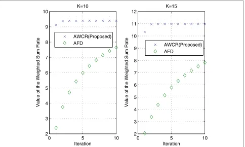
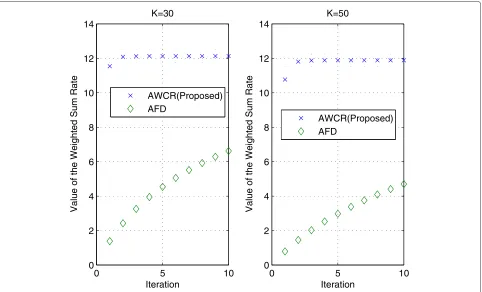
Figures 2 and 3 show the evolution of the weighted sum-rate values versus the number of iterations for AWCR and AFD for some choices of the number of users (K). In the calculation, the number of anten-nas at the base station (m) is set to be 4. Chan-nel gain vectors are generated randomly using random m × 1 vectors with each entry drawn independently from the standard Gaussian distribution. {Pk} is the

set of randomly chosen positive numbers. The sum power constraint is Pt = 10 dB. A group of

dif-ferent weights are also generated randomly. In these figures, the cross markers and the diamond markers rep-resent the results of our proposed Algorithms AWCR and AFD, respectively. These results show that the pro-posed Algorithm AWCR exhibits much faster conver-gence rate, especially with an increasing number of users.

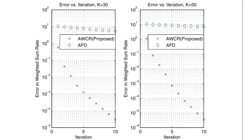
Let f∗ be the maximum sum-rate, f(n) _the sum-rate at the nth iteration and |f(n) _{− f}∗_{| the error in} the sum-rate. Figures 4 and 5 show the correspond-ing error in the sum-rate versus the number of itera-tions. Note it is easy to see that using the fixed-point theory of the proposed Lemma 2 one can determine

the maximum sum-rate f∗ mentioned. As shown in these figures, the algorithms converge linearly. The pro-posed algorithm exhibits a much larger slope in the sum-rate error function, which translates to a faster convergence rate.

We can further observe that the convergence rate of the proposed algorithm is not sensitive to the increase of the number of users. For clearly understanding, we define

NAWCRmin{n| |f(j)−f∗|< f∗, asj≥n},

where the point{(j,f(j))}is generated by the AWCR and

= 10−3 without loss of generality; NAFD is simi-larly defined but generated by the AFD. Each of these numbers can be regarded as the required number of iterations for the corresponding algorithm. We simu-late different selection ofK, and list the corresponding NAWCR and NAFD in Table 1. We can observe that in the simulated range, using the proposed algorithm, the required number of iterations for convergence is about 2, whereas for the AFD, the required number of iterations is much larger.

Since the AFD and the proposed algorithm use the same matrix inverse operations, which consist of the most significant part of the computation, to compute the gradient of the objective values, both algorithms have similar computational complexity O(m3) in each of the iterations (refer to [28]). This is because for a m × m square matrix, its inverse needs m(m2 − 1) + m(m−1)2, i.e.,O(m3), arithmetic operations; its deter-minant needs 2₃m3 + m, i.e., O(m3), operations (the Cholesky decomposition approach is used for efficiency and our objects). Thus, since these operations are used with finite times, it is easily seen that, for each iteration, computational complexities for both AFD and AWCR areO(m3).

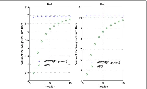
Also for conveniently checking the algorithms, deter-ministic instances are chosen asηk = Kk

k=1k

,∀k,Pt =

10 dB and Pi = 9 dB, ∀i, and the channel gains are

randomly generated as

h†₁,h†₂,h†₃,h†₄

=

⎛

⎝−

0.3864+0.3319i −0.6040+0.3786i 0.3432+0.0937i −0.0561−0.0556i −0.5987−0.6389i −0.8495+0.3909i −0.4211+1.1264i 1.0855−0.4820i −0.1742+0.0254i −0.0848−0.1440i −0.1058+0.7201i −0.4288−0.7245i

0.4688−0.4437i −0.0462−1.4526i −0.3074−1.1175i −0.9527−0.8728i

⎞ ⎠

and

h†₁,h†₂,h₃†,h†₄,h†₅=

⎛ ⎝

0.2042−0.8059i −0.3288+0.4492i −0.9598+0.0608i −0.9767−0.2270i 1.3841−0.8709i −0.3036−0.1493i0.2623−0.4253i −0.7231−1.4174i 0.2231+0.8744i 0.3568+0.7465i

0.0395+0.8416i 0.5150+0.3897i 0.7339−0.3487i 1.0983−0.4464i 1.3184−0.0801i −0.2601−0.7893i1.4935−0.7777i −0.2756+0.3267i 0.5006−1.6442i −0.2403+0.2682i

0 5 10 2

3 4 5 6 7 8 9 10

K=10

Iteration

Value of the Weighted Sum Rate

AWCR(Proposed) AFD

0 5 10

2 3 4 5 6 7 8 9 10 11 12

K=15

Iteration

Value of the Weighted Sum Rate

AWCR(Proposed) AFD

Figure 2Weighted sum-rates (unit: bits) of AWCR and AFD, asK=10 and 15.

forK = 4 andK = 5, respectively. Let the normalized covariances ofC0be the identity matrix. The calculated weighted sum-rate is plotted as a function of the iterations in Figure 6. It is shown that NAWCR=1, keeping the same least value for both cases; andNAFD=10 and 12 asK=4 andK =5, respectively.

6 Conclusion

The proposed algorithm AWCR, as a class of iterative water-filling algorithms, is used to solve the problem of the weighted sum-rate for the MIMO-MAC in a CR net-work. By exploiting the concept of variable weighting factor for covariance update, together with the machinery of distributed and parallel computation, the proposed AWCR algorithm can greatly speed up the convergence rate of the weighted sum-rate maximization computa-tion. The required number of iterations for convergence exhibits non-sensitivity to the increase of the number of the users. Furthermore, a novel GWWFA, as a fundamen-tal block of the proposed algorithm, is proposed.

Convergence of the proposed algorithm is strictly proved by the designed fixed point theory. We present an equivalent optimality condition by Lemma 2, i.e., a point is one of the optimal solutions to the problem of maximum weighted sum-rate for the MISO-MAC in the CR network

if and only if the point is a fixed point of the AWCR. In the derivation, for more general problems, the assumption used in [9] that the optimal solution is unique to prove the convergence could be eliminated. Numerical exam-ples are presented to demonstrate the effectiveness of the proposed algorithm. In the simulated range, the required number of iterations for convergence is shown to be fixed at two, which is a significant reduction compared with the conventional algorithms.

Appendix 1 Proof of Lemma 1

Note that in the following proof, we use the notationnto stand for the number of iterations for convenience.

The necessity is proved first. For the limit(S1,. . .,SK)

of any convergent subsequence, there is a convergent sub-sequence (S(nk)

1 ,. . .,S (nk) K )

!∞

k=0(⊂ (S (n) 1 ,. . .,S

(n)

K )

!∞ n=0) such that

(S1,. . .,SK)=limk→∞(S(nk) 1 ,. . .,S

(nk)

K ), where (S₁(n),. . .,S(_Kn))

!∞ n=0

0 5 10

Value of the Weighted Sum Rate

AWCR(Proposed)

Value of the Weighted Sum Rate

AWCR(Proposed) AFD

Figure 3Weighted sum-rates (unit: bits) of AWCR and AFD, asK=30 and 50.

Assume (S˜(nk+1)

tion of Algorithm AWCR. The definition of Algorithm AWCR implies that

We have the following relationships:

f(S(₁n+1),. . .,S_i−(n+₁1),S_i(n+1),S(_i+n+₁1),. . .,S(_Kn+1))

Among the relationships mentioned above, the first inequality and the first equality hold due to step (3) of Algorithm AWCR; the second inequality results from the

functionf being concave; the third inequality and the sec-ond equality are true because of step (2) of Algorithm AWCR, i.e., the definition of(S˜(₁n+1),. . .,S˜(_Kn+1)).

approach infinity, we may acquire that

0 5 10 10−10

10−8 10−6 10−4 10−2 100 102

Error vs. Iteration, K=10

Iteration

Error in Weighted Sum Rate

AWCR(Proposed) AFD

0 5 10

10−7 10−6 10−5 10−4 10−3 10−2 10−1 100 101

Error vs. Iteration, K=15

Iteration

Error in Weighted Sum Rate

AWCR(Proposed) AFD

Figure 4Error functions of AWCR and AFD, asK=10 and 15.

0 5 10

10−5 10−4 10−3 10−2 10−1 100 101 102

Error vs. Iteration, K=30

Iteration

Error in Weighted Sum Rate

AWCR(Proposed) AFD

0 5 10

10−6 10−5 10−4 10−3 10−2 10−1 100 101 102

Error vs. Iteration, K=50

Iteration

Error in Weighted Sum Rate

AWCR(Proposed) AFD

Table 1 Comparison of the convergence rate

K m=4 m=4

NAWCR NAFD

10 1 27

15 2 39

20 2 54

25 2 65

30 2 79

50 2 133

60 2 159

80 2 n/a

100 2 n/a

110 2 n/a

Note that the set arg max(S1,...,SK)∈Vd

K

i=1f(S1,. . .,Si−1, Si,Si+1,. . .,SK) does not need to be a

single-point set. However, we may choose (S1,. . .,SK)

as one of the optimal solutions to the problem max(S1,...,SK)∈Vd

_K

i=1f(S1,. . .,Si−1,Si,Si+1,. . .,SK). This

corresponds to step (2) of Algorithm AWCR. Further,

(S1,. . .,SK) = β∗(S1,. . .,SK) + (1 − β∗)(S1,. . .,SK),

based on the choice of the optimal solution mentioned above. This corresponds to step (3) of Algorithm AWCR.

Therefore, resulting from the two correspondences mentioned above and the definition of Algorithm AWCR, it is true that(S1,. . .,SK)is a fixed point under Algorithm

AWCR, which is viewed as a mapping. The sufficiency will be proved as follows:

If (S1,. . .,SK) is a fixed point under Algorithm

AWCR, it is seen that if (S(₁0),. . .,S(_K0)) is denoted by

(S1,. . .,SK), then (S(11),. . .,S (1)

K ) = (S1,. . .,SK), i.e.,

the former is assigned by the latter, due to(S1,. . .,SK)

being a fixed point under Algorithm AWCR. If it is assumed that (S(₁n),. . .,S_K(n)) = (S1,. . .,SK), then (S(₁n+1),. . .,S(_Kn+1)) = (S1,. . .,SK) due to (S1,. . .,SK)

being a fixed point under Algorithm AWCR. Accord-ing to the principle of mathematical induction,

(S(₁n),. . .,S_K(n)) = (S1,. . .,SK) ∈ Vd,∀n. Furthermore,

limn→∞(S(₁n),. . .,S_K(n)) = (S1,. . .,SK) ∈ Vd. Therefore,

the sufficiency is true.

Note that in the proving process above, we do not have the following assumption:

(S1,. . .,SK)= lim k→∞(S

(nk+1) 1 ,. . .,S

(nk+1) K ).

Appendix 2 Proof of Lemma 2

The necessity is proved first.

0 5 10

3 3.5 4 4.5 5 5.5 6 6.5 7 7.5

K=4

Iteration

Value of the Weighted Sum Rate AWCR(Proposed)

AFD

0 5 10

4 5 6 7 8 9 10 11

K=5

Iteration

Value of the Weighted Sum Rate AWCR(Proposed)

AFD

According to definition of Algorithm AWCR, it is easily known, for the fixed point(S1,. . .,SK)∈Vd, that

(S1,. . .,SK)∈max(S1,...,SK)∈Vd

×K

i=1f(S1,. . .,Si−1,Si,Si+1,. . .,SK),

where(S1,. . .,SK)∈Vd.

(31)

Since (31) is a convex optimization problem with a con-cave objective function, noting the optimality condition (refer to [29], Proposition 3.1), which is necessary and sufficient for (31), of the convex optimization problems, formula (31) implies that

"

fS1

"

S1,. . .,SK

#

,. . .,fSK

"

S1,. . .,SK

##

·

"

(S1−S1),. . .,(SK−SK)

#T

≤0,

(32)

where,∀(S1,S2,. . .,SK) ∈ Vd, we denote a transpose of

the gradient with respect to the variablesSioff by the row

vectorfSi.

It is seen that formula (32) is just the optimal condition of the optimization problem (3). Therefore, the fixed point

(S1,. . .,SK) ∈ Vd is one of the optimal solutions to the

problem in (3).

The sufficiency will be proved as follows:

_K

i=1f(S1,. . .,Si−1,Si,Si+1,. . .,SK)

=KK_i=1K1f(S1,. . .,Si−1,Si,Si+1,. . .,SK)

≤Kf(_K1(S1,. . .,SK)+ K−_K1(S1,. . .,SK))

≤Kf(S1,. . .,SK)=K_i=1f(S1,. . .,SK).

Among the relationships mentioned above, due to

(S1,. . .,SK) ∈ Vd, the first equality holds; because the

functionf is concave and the set of feasible solutionsVdis

convex, the first inequality holds; since(S1,. . .,SK)∈Vd

is the optimal solution to the problem in (3), the second inequality is true.

Hence,K_i=1f(S1,. . .,Si−1,Si,Si+1,. . .,SK)≤

K

i=1f(S1,. . .,SK),∀(S1,. . .,SK)∈Vd.

According to definition of the optimal solution to (20) mentioned above,

(S1,. . .,SK)∈arg max(S1,...,SK)∈Vd

K

i=1

f(S1,. . .,Si−1,Si,Si+1,. . .,SK).

According to steps (2) and (3) of Algorithm AWCR,

(S1,. . .,SK) ∈ Vd is a fixed point under Algorithm

AWCR.

Competing interests

The authors declare that they have no competing interests.

Acknowledgements

The authors sincerely acknowledge the support from Natural Sciences and Engineering Research Council (NSERC) of Canada under grant number RGPIN/293237-2009, National Natural Science Foundation of China (NSFC) under grant number 61021001, and Tsinghua National Laboratory for Information Science and Technology (TNList). The authors were grateful to the anonymous reviewers and guest editors for their valuable comments and suggestions to improve the quality of the article.

Author details

1_{Department of Electrical and Computer Engineering, Ryerson University,} Ontario,M5B 2K3, Canada.2_{Department of Electronic Engineering, Tsinghua} University, Beijing, 100084, China.

Received: 2 June 2012 Accepted: 1 February 2013 Published: 17 April 2013

References

1. H Jiang, L Lai, R Fan, HV Poor, Optimal selection of channel sensing order in cognitive radio. IEEE Trans. Wirel. Commun.8, 297–307 (2009) 2. RV Prasad, P Pawelczak, JA Hoffmeyer, HS Berger, Cognitive functionality

in next generation wireless networks: standardization efforts. IEEE Commun. Mag.46, 72–78 (2008)

3. J Mitola, GQ Maguire, Cognitive radios: making software radios more personal. IEEE Personal Commun.6, 13–18 (1999)

4. S Haykin, Cognitive radio: brain-empowered wireless communications. IEEE J. Sel. Areas Commun.23, 201–220 (2005)

5. N Devroye, M Vu, V Tarokh, Cognitive radio networks: Information theory limits, models and design. IEEE Signal Process. Mag.25,

12–23 (2008)

6. E Biglieri, R Calderbank, A Constantinides, A Goldsmith, A Paulraj, HV Poor, MIMO Wireless Communications(Cambridge University Press,

Cambridge, 2007)

7. D Tse, S Hanly, Multiaccess fading channels. Part I: Polymatroid structure, optimal resource allocation and throughput capacities. IEEE Trans. Inf. Theory44, 2796–2815 (1998)

8. S Vishwanath, S Jafar, A Goldsmith, Optimum power and rate allocation strategies for multiple access fading channels,in Proc. IEEE Vehicular Technology Conf.(Rhodes, 2001) pp. 2888–2892

9. N Jindal, W Rhee, S Vishwanath, SA Jafar, A Goldsmith, Sum power iterative water-filling for multi-antenna Gaussian broadcast channels. IEEE Trans. Inf. Theory51, 1570–1580 (2005)

10. W Yu, Sum-capacity computation for the Gaussian vector broadcast channel via dual decomposition. IEEE Trans. Inf. Theory52, 754–759 (2006)

11. W Yu, W Rhee, S Boyd, JM Cioffi, Iterative water-filling for Gaussian vector multi-access channels. IEEE Trans. Inf. Theory50, 145–152,

(2004)

12. E Telatar, Capacity of multi-antenna Gaussian channels. Europ. Trans. Telecommun.10, 585–596 (1999)

13. N Jindal, S Vishwanath, A Goldsmith, On the duality of Gaussian multiple-access and broadcast channels. IEEE Trans. Inf. Theory 50, 768–783 (2004)

14. P Viswanath, D Tse, Sum capacity of the multiple antenna Gaussian broadcast channel and uplink-downlink duality. IEEE Trans. Inf. Theory 49, 1912–1921 (2003)

15. H Weingarten, Y Steinberg, S Shamai, The capacity region of the Gaussian multiple-input multiple-output broadcast channel. IEEE Trans. Inf. Theory 52, 3936–3964 (2006)

16. M Kobayashi, G Caire, An iterative water-filling algorithm for maximum weighted sum-rate of Gaussian MIMO-BC. IEEE J. Sel. Areas Commun. 24, 1640–1646 (2006)

17. L Zhang, Y-C Liang, Y Xin, Joint beamforming and power allocation for multiple access channels in cognitive radio networks. IEEE J. Sel. Areas Commun.26, 38–51 (2008)

19. R Zhang, S Cui, YC Liang, On ergodic sum capacity of fading cognitive multiple-access and broadcast channels. IEEE Trans. Inf. Theory 55, 5161–5178 (2009)

20. D Palomar, Practical algorithms for a family of waterfilling solutions. IEEE Trans. Signal Process.53, 686–695 (2005)

21. C Hs, H Su, P Lin, Joint subcarrier pairing and power allocation for OFDM transmission with decode-and-forward relaying. IEEE Trans. Inf. Theory 59, 399–414 (2011)

22. Q Qi, A Minturn, Y Yang, An efficient water-filling algorithm for power allocation in OFDM-based cognitive radio systems. inProc. International Conference on Systems and Informatics (ICSAI)(Yantai, 2012) pp. 2069–2073 23. Y Rong, X Tang, Y Hua, A unified framework for optimizing linear

non-regenerative multicarrier MIMO relay communication systems. IEEE Trans. Signal Process.57, 4837–4852 (2009)

24. A Quarteroni, R Sacco, F Saleri,Numerical Mathematics, 2nd edn., (Springer, Berlin Heidelberg, 2010)

25. P He, L Zhao, Correction of convergence proof for iterative water-filling in Gaussian MIMO broadcast channels. IEEE Trans. Inf. Theory57, 2539–2543 (2011)

26. W Zangwill,Nonlinear Programming: A Unified Approach(Prentice-Hall, Englewood Cliffs, 1969)

27. W Sun, Y Yuan,Optimization Theory and Methods: Nonlinear Programming, 1st edn., (Springer Optimization and Its Applications). (Springer, New York, 2006)

28. CH Papadimitriou, K Steiglitz,Combinatorial Optimization: Algorithms and Complexity, Unabridged edition. (Dover Publications, Mineola, 1998) 29. DP Bertsekas, JN Tsitsiklis,Parallel and Distribution Computation: Numerical

Methods, 1st edn. (Athena Scientific, Nashua, 1997)

doi:10.1186/1687-6180-2013-80

Cite this article as:Heet al.:Weighted sum-rate maximization for multi-user SIMO multiple access channels in cognitive radio networks.EURASIP

Journal on Advances in Signal Processing20132013:80.

Submit your manuscript to a

journal and benefi t from:

7Convenient online submission

7Rigorous peer review

7Immediate publication on acceptance

7Open access: articles freely available online

7High visibility within the fi eld

7Retaining the copyright to your article