Grounded Textual Entailment

2354

Grounded Textual Entailment

Hoa Trong Vu∗+, Claudio Greco†, Aliia Erofeeva†+, Somayeh Jafaritazehjan∗+ Guido Linders†+, Marc Tanti∗, Alberto Testoni†, Raffaella Bernardi†, Albert Gatt∗

+_{Erasmus Mundus European Program in Language and Communication Technology}

∗_{University of Malta,}†_{University of Trento}

∗_{name.surname@um.edu.mt,}†_{name.surname@unitn.it}

Abstract

Capturing semantic relations between sentences, such as entailment, is a long-standing challenge for computational semantics. Logic-based models analyse entailment in terms of possible worlds (interpretations, or situations) where a premise P entails a hypothesis H iff in all worlds where P is true, H is also true. Statistical models view this relationship probabilistically, addressing it in terms of whether a human would likely infer H from P. In this paper, we wish to bridge these two perspectives, by arguing for a visually-grounded version of the Textual Entailment task. Specifically, we ask whether models can perform better if, in addition to P and H, there is also an image (corresponding to the relevant “world” or “situation”). We use a multimodal version of the SNLI dataset (Bowman et al., 2015) and we compare “blind” and visually-augmented models of textual entailment. We show that visual information is beneficial, but we also conduct an in-depth error analysis that reveals that current multimodal models are not performing “grounding” in an optimal fashion.

1 Introduction

Evaluating the ability to infer information from a text is a crucial test of the capability of models to grasp meaning. As a result, the computational linguistics community has invested huge efforts into developing textual entailment (TE) datasets.

After formal semanticists developed FraCas in the mid ’90 (Cooper et al., 1996), an increase in statisti-cal approaches to computational semantics gave rise to the need for suitable evaluation datasets. Hence, Recognizing Textual Entailment (RTE) shared tasks have been organized regularly (Sammons et al., 2012). Recent work on compositional distributional models has motivated the development of the SICK dataset of sentence pairs in entailment relations for evaluating such models (Marelli et al., 2014). Fur-ther advances with Neural Networks (NNs) have once more motivated efforts to develop a large natural language inference dataset, SNLI (Bowman et al., 2015), since NNs need to be trained on big data.

However, meaning is not something we obtain just from text and the ability to reason is not unimodal either. The importance of enriching meaning representations with other modalities has been advocated by cognitive scientists, (e.g., (Andrews et al., 2009; Barsalou, 2010)) and computational linguists (e.g., (Glavaˇs et al., 2017)). While efforts have been put into developing multimodal datasets for the task of checking Semantic Text Similarity Text (Agirre et al., 2017), we are not aware of any available datasets to tackle the problem of Grounded Textual Entailment (GTE). Our paper is a first effort in this direction. Textual Entailment is defined in terms of the likelihood of two sentences (a premise P and an hypoth-esis H) to be in a certain relation: P entails, contradicts or is unrelated to H. For instance, the premise “People trying to get warm in front of a chimney” and the hypothesis “People trying to get warm at home” are highly likely to be in an entailment relation. Our question is whether having an image that illustrates the event (e.g., Figure 1a) can help a model to capture the relation. In order to answer this

Correspondence should be addressed to Raffaella Bernardi (raffaella.bernardi@unitn.it) and Albert Gatt (albert.gatt@um.edu.mt).

This work is licensed under a Creative Commons Attribution 4.0 International License. License details:

http://creativecommons.org/licenses/by/4.0/. The dataset, annotation and code is available from

(a) P:A family in front of a chimneyand H:A family trying to get warm

(b) P:People trying to get warmand H:People are out-side on a chilly day. TE: unrelated vs. GTE: related

Figure 1: Premise, Hypothesis and Image examples

question, we augment the largest available TE dataset with images, we enhance a state of the art model of textual entailment to take images into account and we evaluate it against the GTE task.

The inclusion of images can also alter relations which, based on text alone, would seem likely. For example, to a “blind” model the sentences of the sentence pair in Figure 1b would seem to be unrelated, but when the two sentences are viewed in the context of the image, they do become related.

A suitable GTE model therefore has to perform two sub-tasks: (a) it needs to ground its linguistic representations of P, H or both in non-linguistic (visual) data; (b) it needs to reason about the possible relationship between P and H (modulo the visual information).

2 Related Work

Grounding language through vision has recently become the focus of several tasks, including Image Captioning (IC, e.g. (Hodosh et al., 2013; Xu et al., 2015)) and Visual Question Answering (VQA, eg. (Malinowski and Fritz, 2014; Antol et al., 2015)), and even more recently, Visual Reasoning (Johnson et al., 2017; Suhr et al., 2017) and Visual Dialog (Das et al., 2017). Our focus is on Grounded Textual Entailment (GTE). While the literature on TE is rather vast, GTE is still rather unexplored territory.

Textual Entailment Throughout the history of Computational Linguistics various datasets have been built to evaluate Computational Semantics models on the TE task. Usually they contain data divided into entailment, contradiction or unknown classes. The “unknown” label has sometimes been replaced with the “unrelated” or “neutral” label, capturing slightly different types of phenomena. Interestingly, the “entailment” and “contradiction” classes also differ across datasets. In the mid-’90s a group of formal semanticists developed FraCaS (Framework for Computational Semantics). (Cooper et al., 1996)1 The dataset contains logical entailment problems in which a conclusion has to be derived from one or more premises (but not necessarily all premises are needed to verify the entailment). The entailments are driven by logical properties of linguistic expressions, like the monotonicity of quantifiers, or their conservativity property etc. Hence, the set of premises entails the conclusion iff in all the interpretations (worlds) in which the premises are true the conclusion is also true; otherwise the conclusion contradicts the premises. In 2005, the PASCAL RTE (Recognizing Textual Entailment) challenge was launched, to become a task organized annually. In 2008, the RTE-4 committee made the task more fine-grained by requiring the classification of the pairs as “entailment”, “contradiction” and “unknown” (Giampiccolo et al., 2008). The RTE datasets, unlike FraCaS, contain real-life natural language sentences and the sort of entailment problems which occur in corpora collected from the web. Importantly, the sentence pair relations are annotated as entailment, contradiction or neutral based on a likelihood condition: if a human reading the premise would typically infer that the conclusion (called the hypothesis) is most likely true (entailment), its negation is most likely true (contradiction) or the conclusion can be either true or false (neutral).

At SemEval 2014, in order to evaluate Compositional Distributional Semantics Models focusing on the compositionality ability of those models, the SICK dataset (Sentences Involving Compositional Knowl-edge) was used in a shared entailment task (Marelli et al., 2014). Sentence pairs were obtained through

re-writing rules and annotated with the three RTE labels via a crowdsourcing platform. Both in RTE and SICK the label assigned to the sentence pairs captures the relation holding between the two sentences.

A different approach has been used to build the much larger SNLI (Stanford Natural Language In-ference) dataset (Bowman et al., 2015): Premises are taken from a dataset of images annotated with descriptive captions; the corresponding hypotheses were produced through crowdsourcing, where for a given premise, annotators provided a sentence which is true or not true with respect to a possible image which the premise could describe. A consequence of this choice is that the contradiction relation can be assigned to pairs which are rather unrelated (“A person in a black wetsuit is surfing a small wave” and “A woman is trying to sleep on her bed”), differently from what happens in RTE and SICK.

Since the inception of RTE shared tasks, there has been an increasing emphasis on data-driven ap-proaches which, given the hypothesis H and premise P, seek to classify the semantic relation (see (Sam-mons et al., 2012) for a review). More recently, neural approaches have come to dominate the scene, as shown by the recent RepEval 2017 task (Nangia et al., 2017), where all submissions relied on bidi-rectional LSTM models, with or without pretrained embeddings. RTE also intersects with a number of related inference problems, including semantic text similarity and Question Answering, and some mod-els have been proposed to address several such problems. In one popular approach, both P and H are encoded within the same embedding space, using a single RNN, with a decision made based on the en-codings of the two sentences. This is the approach we adopt for our baseline LSTM in Section 4, based on the model proposed by Bowman et al. (2015), albeit with some modifications (see also (Tan et al., 2016)). A second promising approach, based on which we adapt our state of the art model, relies on matching and aggregation (Wang et al., 2017). Here, the decision concerning the relationship between P and H is based on an aggregate representation achieved after the two sentences are matched. Yet another area where neural approaches are being applied to sentence pairs in an entailment relationship is genera-tion, where an RNN generates an entailed hypothesis (or a chain of such hypotheses) given an encoding of the premise (Kolesnyk et al., 2016; Starc and Mladeni´c, 2017).

Vision and Textual Entailment In recent years, several models have been proposed to integrate the language and vision modalities; usually the integration is operationalized by element-wise multiplication between linguistic and visual vectors. Though the interest in these modalities has spread in an astonish-ing way thanks to various multimodal tasks proposed, includastonish-ing the IC, VQA, Visual Reasonastonish-ing and Visual Dialogue tasks mentioned above, very little work has been done on grounding entailment. In-terestingly, Young et al. (2014) has proposed the idea of considering images as the “possible worlds” on which sentences find their denotation. Hence, they released a “visual denotation graph” which asso-ciates sentences with their denotation (sets of images). The idea has been further exploited by Lai and Hockenmaier (2017) and Han et al. (2017). Vendrov et al. (2016) look at hypernymy, textual entailment and image captioning as special cases of a single visual-semantic hierarchy over words, sentences and images, and they claim that modelling the partial order structure of this hierarchy in visual and linguistic semantic spaces improves model performance on those three tasks.

We share with this work the idea that the image can be taken as a possible world. However, we don’t use sets of images to obtain the visual denotation of text in order to check whether entailment is logically valid/highly likely. Rather, we take the image to be the world/situation in which the text finds its interpretation. The only work that is close to ours is an unpublished student report (Sitzmann et al., 2016), which however lacks the in-depth analysis presented here.

3 Annotated dataset of images and sentence pairs

test set, but then zoom in on SNLIhardto understand the models’ behaviour. We briefly introduce SNLI and the new test set and compare them through our annotation of linguistic phenomena.

3.1 Dataset construction

SNLI and SNLIhard test set The SNLI dataset (Bowman et al., 2015) was built through Amazon Mechanical Turk. Workers were shown captions of photographs without the photo and were asked to write a new caption that (a) is definitely a true description of the photo (entailment); (b) might be a true description of the photo (neutral); (c) is definitely a false description of the photo (contradiction). Examples were provided for each of the three cases. The premises are captions which come mostly from Flickr30K (Young et al., 2014); only 4K captions are from VisualGenome (Krishna et al., 2017). In total, the dataset contains 570,152 sentence pairs, balanced with respect to the three labels. Around 10% of these data have been validated (4 annotators for each example plus the label assigned through the previous data collection phase). The development and test datasets contain 10K examples each. Moreover, each Image/Flickr caption occurs in only one of the three sets, and all the examples in the development and test sets have been validated.

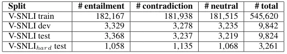
V-SNLI and V-SNLIhardtest set Our grounded version of SNLI, V-SNLI, has been built by matching each sentence pair in SNLI with the corresponding image coming from the Flickr30K dataset; thus the V-SNLI dataset is slightly smaller than the original, which also contains captions from VisualGenome. V-SNLI consists of 565,286 pairs (187,969 neutral, 188,453 contradiction, and 188,864 entailment). Training, test, and development splits have been built according to the splits in SNLI. The main statistics of the splits of the dataset are reported in Table 1 together with statistics for the visual counterpart of Hard SNLI, namely V-SNLIhard. By construction, V-SNLI contains datapoints such that the premise is always true with respect to the image, whereas the hypothesis can be either true (entailment or neutral cases) or false (contradiction or neutral cases.)

Split # entailment # contradiction # neutral # total

V-SNLI train 182,167 181,938 181,515 545,620

V-SNLI dev 3,329 3,278 3,235 9,842

V-SNLI test 3,368 3,237 3,219 9,824

V-SNLIhardtest 1,058 1,135 1,068 3,261

Table 1: Statistics of the V-SNLI dataset.

3.2 Dataset annotation

For deeper analysis and comparison of the contents of SNLI and SNLIhard, we have annotated the SNLI dataset by both automatically detecting some surface linguistic cues and manually labelling less trivial phenomena. Using an in-house annotation interface, we collected human judgments aiming to (a) filter out those cases for which the gold-standard annotation was considered to be wrong2; (b) connect the three ungrounded relations to various linguistic phenomena. To achieve this, we annotated a random sample of the SNLI test set containing 527 sentence pairs (185 entailment, 171 contradiction, 171 neutral), out of which 176 were from the hard test set (56 entailment, 62 contradiction, 58 neutral).

All the pairs were annotated by at least two annotators, as follows: (a) We filtered out all the pairs which had a wrong gold label (see Table 2 for details). When our annotators did not agree whether a given relation holds for a specific pair, we appealed to the corresponding five judgments coming from the validation stage of the SNLI dataset to reach a consensus based on the majority of labels. (b) We considered as valid any linguistic tag assigned by at least one annotator. Since the annotation for (a) is binary whereas for (b) it is multi-class, we used Cohen’s κ for the former and also Scott’s π and Krippendorff’sα for the latter as suggested by Passonneau (2006). The inter-annotator agreement for the relation type (a) wasκ= 0.93; for (b) linguistic tags it wasπ = 0.63,α= 0.61, andκ= 0.643.

2

An example of a wrong annotation is the pairA white greyhound dog wearing a muzzle runs around a trackandThe dog is racing other dogs, labelled as entailment in the SNLI test set.

Ungrounded Grounded

entailment contradiction neutral entailment contradiction neutral

SNLI 7% 16% 2% 1% 1% 31%

SNLIhard 6% 10% 1% <1% 1% 20%

Table 2: Wrong gold-standard labels: Data for which the gold standard label was considered to be wrong (a) in theungrounded setting or (b) correct in the ungrounded setting but not in thegroundedone. We filter out the data in (a) and keep those in (b).

Tag Description Example

Paraphrase Two-way entailment, i.e., H entails P and vice versa.

P:A middle eastern marketplace, H:A middle east-ern store

Generalisation One-way entailment, i.e., H entails P but not nec-essarily vice versa.

P:A group of people on the beach with cameras, H:People are on a beach.

Entity P and H describe different entities (e.g., subject, object, location) or incompatible properties of en-tities (e.g., color).

P:A dog runs along the ocean surf, H:A cat is running in the waves.

Verb The sentences describe different, incompatible ac-tions.

P:Military personnel are shopping, H:People in the military are training.

Insertion H contains details and facts not present in P (e.g., subjective judgments and emotions.)

P:Woman reading a book in a laundry room, H:

The book is old.

Unrelated The sentences are completely unrelated. P: A woman is applying lip makeup to another woman, H:The man is ready to fight.

Quantifier The sentences contain numbers or quantifiers (e.g.,

all, no, some, both, group).

P:A group of people are taking a fun train ride, H:

People ride the train. World knowledge Commonsense assumptions are needed to

under-stand the relation between sentences (e.g., if there are named entities).

P:A crowd gathered on either side of a Soap Box Derby, H:The people are at the race.

Voice The premise is an active/passive transformation of the hypothesis.

P:Kids being walked by an adult, H:An adult is escorting some children.

Swap The sentences’ subject and object are swapped from P to H.

P:A woman walks in front of a giant clock, H:The clock walks in front of the woman.

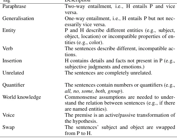
Table 3: Tags used in manual annotation of a subset of the SNLI test set.

Linguistic phenomena Following the error analysis approach described in recent work (Nangia et al., 2017; Williams et al., 2018), we compiled a new list of linguistic features that can be of interest when contrasting SNLI and SNLIhard, as well as for evaluating RTE models. Some of these were detected automatically, while others were assigned manually. Automatic tags included SYNONYM and ANTONYM, which were detected using WordNet (Miller, 1995). QUANTIFIER, PRONOUN, DIFFTENSE, SUPERLATIVE and BARE NP were identified using Penn treebank labels (Marcus et al., 1993), while labels such as NEGATIONwere found with a straightforward keyword search. The tag LONGhas been assigned to sentence pairs with a premise containing more than 30 tokens, or a hypothesis with more than 16 tokens. Details about the tags used in the manual annotation are presented in Table 3.

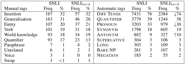
We examined the differences in the tags distributions between the SNLI and SNLIhardtest sets (Ta-ble 4). Interestingly, the hard sentence pairs from our random sample include proportionately more antonyms but fewer pronouns, as well as examples with different verb tenses in the premise and hypoth-esis, compared to the full test set. Furthermore, SNLIhard contains a significantly larger proportion of gold-standard labels which become wrong when the image is factored in (χ2-test withα= 0.05).

4 Models

In this section, we describe a variety of models that were compared on both V-SNLI and V-SNLIhard, ranging from baseline models based on Bowman et al. (2015) to a state of the art model by Wang et al. (2017). We compare the original ‘blind’ version of a model with a visually-augmented counterpart. In what follows, we usePandHto refer to a premise and hypothesis, respectively.

SNLI SNLIhard SNLI SNLIhard

Manual tags Freq % Freq % Automatic tags Freq % Freq % Insertion 167 32 57 32 DIFFTENSE 7431 76 2384 ↓74 Generalisation 163 31 46 26 QUANTIFIER 3779 39 1244 38 Entity 107 20 37 21 PRONOUN 3203 33 979 ↓30

Verb 101 19 31 18 SYNONYM 1798 18 605 19

World knowledge 93 18 34 19 ANTONYM 882 9 327 ↑10 Quantifier 91 17 23 13 SUPERLATIVE 304 3 106 3

Paraphrase 7 1 4 2 LONG 303 3 109 3

Unrelated 6 1 2 1 BARENP 281 3 107 3

Voice 3 1 0 0 NEGATION 185 2 55 2

Swap 1 <1 1 1

Table 4: Distribution of the automatic and manually assigned tags in the SNLI and SNLIhardtest sets. Automatic tags are detected in the whole test set, manual ones are assigned to its random subset. Arrows

↑↓signify a statistically significant difference in tag proportions between the datasets (Pearson’sχ2-test).

are then concatenated in a stack of three 512D layers having a ReLU activation function (Nair and Hinton, 2010), with a final softmax layer to classify the relation between the two sentences as entailment, contra-diction or neutral. The model is inspired by the LSTM baseline proposed by Bowman et al. (2015)4. The model exploits the 300,000 most frequent pretrained GloVe embeddings (Pennington et al., 2014) and improves them during the training process. To regularize the model, Dropout (Srivastava et al., 2014) is applied to the inputs and outputs of the recurrent layers and to the ReLU fully connected layers with a keeping probability of 0.5. The model is trained using the Adam optimizer (Kingma and Ba, 2014) with a learning rate of 0.001 until its accuracy on the development set drops for three successive iterations.

V-LSTM baseline The LSTM model described above is augmented with a visual component following a standard Visual Question Answering baseline model (Antol et al., 2015). Following initial representa-tion of P and H in 512D vectors through an LSTM, a fully-connected layer projects the L2-normalized 4096D image vector coming from the penultimate layer of a VGGnet16 Convolutional Neural Net-work (Simonyan and Zisserman, 2014) to a reduced 512D vector. A fully-connected layer with a ReLU activation function is also applied to P and H to obtain two 512D vectors. The multimodal fusion between the text and the image is obtained by performing an element-wise multiplication between the vector of the text representation and the reduced vector of the image. The multimodal fusion is performed between the image and both the premise and the hypothesis, resulting in two multimodal representations. The re-lation between them is captured as in the model described above. This model uses GloVe embeddings and the same optimization and procedure described above.

We have also adapted a state-of-the-art attention-based model for IC and VQA (Anderson et al., 2017; Teney et al., 2017) to the GTE task. It obtains results comparable to the V-LSTM. This lack of improve-ment might be due to the need of further parameter tuning. We report the details of our impleimprove-mentation and its results in the Supplementary Material.

BiMPM The Bilateral Multi-Perspective Matching (BiMPM) model (Wang et al., 2017) obtains state-of-the-art performance on the SNLI dataset, achieving a maximum accuracy of 86.9%, and going up to 88.8% in an ensemble setup. An initial embedding layer vectorises words in P and H using pretrained GLoVe embeddings (Pennington et al., 2014), and passing them to a context representation layer, which uses bidirectional LSTMs (BiLSTMs) to encode context vectors for each time-step. The core part of the model is the subsequent matching layer, where each contextual embedding or time-step of P is matched against all the embeddings of H, and vice versa. The output of this layer is composed of two sequences of matching vectors, which constitute the input to another BiLSTM at the aggregation layer. The vectors from the last time-step of the BiLSTM are concatenated into a fixed-length vector, which is passed to the final prediction tier, a two-layer feed-forward network which classifies the relation between P and H

4_{There are some differences between our baseline and the LSTM baseline used in (Bowman et al., 2015). In particular,}

LSTM [H] LSTM V-LSTM BiMPM V-BiMPM Entailment 72.65 87.71 87.14 90.03 90.38 Contradiction 66.29 79.7 71.39 86.25 87.53 Neutral 66.36 76.79 68.06 82.79 82.91 Overall 68.49 81.49 75.70 86.41 86.99

Table 5: Accuracies (%) for V-SNLI. [H] indicates a baseline model encoding only the hypothesis.

LSTM [H] LSTM V-LSTM BiMPM V-BiMPM Entailment 31.28 72.12 69.09 80.43 81.38 Contradiction 25.29 60.79 46.34 77.62 76.12 Neutral 20.22 50.19 32.02 59.36 63.67 Overall 25.57 60.99 49.03 72.55 73.75

Table 6: Accuracies (%) for V-SNLIhard. [H] indicates a baseline model encoding only the hypothesis.

via softmax. Matching is performed via a cosine operation, which yields anl-dimensional vector, where

lis the number of perspectives. Wang et al. (2017) experiment with four different matching strategies. In their results, the best-performing version of the BiMPM model used all four matching strategies. We adopt this version of the model in what follows.

V-BiMPM model We enhanced BiMPM to account for the image, too. Our version of this model is referred to as theV-BiMPM. Here, the feature vector for an image is obtained from the layer before the fully-connected layer of a VGGnet-16. This results in a7×7×512tensor, which we consider as 49 512-dimensional vectors. The same matching operations are performed, except that matching occurs between P, H, and the image. Since the textual and visual vectors have different dimensionality and belong to different spaces, we first map them to a mutual space using an affine transformation. We match textual and image vectors using a cosine operation, as before. Full details of the model are reported in the Supplementary Materials for this paper.

5 Experiments and Results

The models described in the previous sections were evaluated on both (V-)SNLI and (V-)SNLIhard. For the visually-augmented models, we experimented with configurations where image vectors were combined with both P and H (namely P+I and H+I), or only with H (P and H+I). The best setting was invariably the one where only H was grounded; hence, we focus on these results in what follows, comparing them to “blind” models. In view of recent results suggesting that biases in SNLI afford a high accuracy in the prediction task with only the hypothesis sentence as input (Gururangan et al., 2018), we also include results for the blind models without the premise (denoted with [H] in what follows).

Table 5 shows the results of the various models on the full V-SNLI dataset. The same models are compared in Table 6 on V-SNLIhard. First, note that the LSTM [H] model evinces a drop in performance compared to LSTM (from 81.49% to 68.49%), though the drop is much greater on the unbiased SNLIhard subset (from 60.99 to 25.57%). This confirms the results reported by Gururangan et al. (2018) and justifies our additional focus on this subset of the data.

The effect of grounding in these models is less clear. The LSTM baseline performs worse when it is visually augmented; this is the case of V-SNLI and, even more drastically, V-SNLIhard. It is also true irrespective of the relationship type. On the other hand, the V-BiMPM model improves marginally across the board, compared to BiMPM, on the V-SNLI data. On the hard subset, the images appear to hurt performance somewhat in the case of contradiction (from 77.62% to 76.12%), but improve it by a substantial margin on neutral cases (from 59.36% to 63.67%). The neutral case is the hardest for all models, with the possible exception of LSTM [H] on the full dataset.

turn to a more detailed error analysis of the V-BiMPM model, first in relation to the dataset annotations, and then by zooming in somewhat closer on V-SNLIhard.

5.1 Error analysis by linguistic annotation label

Manual tags BiMPM V-BiMPM Automatic tags BiMPM V-BiMPM

Insertion 58 63 ANTONYM 84 84

Generalisation 93 89 BARENP 79 75

Entity 95 ↓78 QUANTIFIER 73 73

Verb 77 68 DIFFTENSE 72 73

World knowledge 79 71 PRONOUN 69 70

Quantifier 78 70 SYNONYM 69 71

Paraphrase 75 75 LONG 67 73

Unrelated 50 50 SUPERLATIVE 64 63

Swap 0 0 NEGATION 51 56

Table 7: Accuracies obtained by BiMPM and V-BiMPM models on SNLIhard, by annotation tags. Ar-rows ↑↓signify a statistically significant difference in tag proportions between the datasets (Pearson’s

χ2-test).

In Table 7, accuracies for the blind and grounded version of BiMPM are broken down by the labels given to the sentence pairs in the annotated subset of SNLI described in Section 3. We only observe a significant difference in theEntitycase, that is, where the referents in P and H are inconsistent. Here, the blind model outperforms the grounded one, an unexpected result, since one would assume a grounded model to be better equipped to identify mismatched referents. Hence, in the following we aim to under-stand whether the models properly deal with the grounding sub-task.

5.2 Error analysis on grounding in the SNLIhard

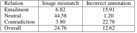
We next turn to the “hard” subset of the data, where V-BiMPM showed some improvement over the blind case, but suffered on contradiction cases (Table 6). We analysed the 207 cases in SNLIhardwhere the V-BiMPM made incorrect predictions compared to the blind model, that is, where the image hurt performance. These were annotated independently by two of the authors (raw inter-annotator agreement: 96%) who (a) read the two sentences, P and H; (b) checked whether the relation annotated in the dataset actually held or whether it was an annotation error; (c) in those cases where it held, checked whether including the image actually resulted in a change in the relation.

Table 8 displays the proportions of image mismatch and incorrect annotations. As the table suggests, in the cases where images hinder performance in the V-BiMPM, it is usually because the image changes the relation (thus, these are cases of image mismatch; see Section 1 for an example); this occurs in a large proportion of cases labelled as neutral in the dataset.

Inspired by the work in (Mironenco et al., 2017), we further explored the impact of visual grounding in both the V-LSTM and V-BiMPM by comparing their performance on SNLIhard, with the same subset incorporating image “foils”. Vectors for the images in the V-SNLI test set were compared pairwise using cosine, and for each test case in V-SNLIhard, the actual image was replaced with the most dissimilar image in the full test set. The rationale is that, if visual grounding is really helpful in recognising the semantic relationship between P and H, we should observe a drop in performance when the images are

Relation Image mismatch Incorrect annotation

Entailment 6.82 15.91

Neutral 44.58 1.20

Contradiction 3.80 22.78

Overall 24.76 12.62

V-LSTM V-BiMPM Original Foil Original Foil Entailment 69.09 65.03 81.38 80.81 Contradiction 46.34 30.92 76.12 74.98 Neutral 32.02 31.46 63.67 63.39 Overal 49.03 46.92 (-2.11) 73.75 73.08 (-0.67)

Table 9: Accuracies of the visually-augmented models on V-SNLIhardwith original or foil image.

V-LSTM V-BiMPM Entailment 40.74 51.89 Contradiction 30.22 40.7 Neutral 22.47 32.02 Overall 31.09 41.49

GT class Prediction V-LSTM V-BiMPM Contradiction Contradiction 343 462 Contradiction *Entailment 442 327 Contradiction Neutral 350 346 Entailment Entailment 431 549 Entailment *Contradiction 254 166 Entailment Neutral 373 343

Neutral Neutral 240 342

Neutral Contradiction 377 263 Neutral Entailment 451 463

Table 10: Confusion matrices for [H+I]. (*) marks implausible errors.

unrelated to the scenario described by the sentences. The results are displayed in Table 9, which also reproduces the original results on V-SNLIhardfrom Table 6 for ease of reference.

As the results show, models are not hurt by the foil image, contrary to our expectations. V-BiMPM overall drops just by 0.67% whereas V-LSTM drop is somewhat higher (-2.11%) showing it might be doing a better job on the grounding sub-task.

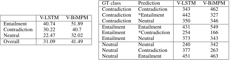
As a final check, we sought to isolate the grounding from the reasoning sub-task, focusing only on the former. We compared the models when grounding only the hypothesis [H+I], while leaving out the premise. Note that this test is different from the evaluation of the model using only the hypothesis [H]: Whereas in that case the input is not expected to provide any useful information to perform the task, here it is. As we noted in Section 3, by construction the premise is always true with respect to the image while the hypothesis can be either true (entailment or neutral cases) or false (contradiction or neutral cases). A model that is grounding the text adequately would be expected to confuse both entailment and contradiction cases with neutral ones; on the other hand, neutral cases should be confused with entailments or contradictions. Confusing contradictions with entailments would be a sign that a model is grounding inadequately, since it is not recognising that H is false with respect to the image.

As the left panel of Table 10 shows, V-BiMPM outperforms V-LSTM by a substantial margin, though the performance of both models drops substantially with this setup. The right panel in the table shows that neither model is free of implausible errors (confusing entailments and contradictions), though V-BiMPM makes substantially fewer of these.

6 Conclusion

This paper has investigated the potential of grounding the textual entailment task in visual data. We argued that a Grounded Textual Entailment model needs to perform two tasks: (a) the grounding itself, and (b) reasoning about the relation between the sentences, against the visual information. Our results suggest that a model based on matching and aggregation like the BiMPM model (Wang et al., 2017) can perform very well at the reasoning task, classifying entailment relations correctly much more frequently than a baseline V-LSTM. On the other hand, it is not clear that grounding is being performed adequately in this model. It is primarily in the case of contradictions that the image seems to play a direct role in biasing the classification towards the right or wrong class, depending on whether the image is correct.

identify a mismatch between the hypothesis and the scene described by the premise, a situation which is rendered opaque by the introduction of foils. Second, in those cases where improvements are observed in the state of the art V-BiMPM, the precise role played by the image is not straightforward. Indeed, we find that this model still marginally outperforms the ‘blind’, text-only model overall, when the images involved are foils rather than actual images.

We believe that further research on grounded TE is worthy of the NLP community’s attention. While linking language with perception is currently a topical issue, there has been relatively little work on linking grounding directly with inference. By drawing closer to a joint solution to the grounding and inference tasks, models will also be better able to address language understanding in the real world.

The present paper presented a first step in this direction using a version of an existing TE dataset which was augmented with images that could be paired directly with the premises, since these were originally captions for those images. However, it is important to note that in this dataset premise-hypotheses pairs were not generated directly with reference to the images themselves. An important issue to consider in future work on GTE, besides the development of better models, is the development of datasets in which the role of perceptual information is controlled, ensuring that the data on which models are trained represents truly grounded inferences.

Acknowledgements

We kindly acknowledge the European Network on Integrating Vision and Language (iV&L Net) ICT COST Action IC1307. Moreover, we thank the Erasmus Mundus European Program in Language and Communication Technology. Marc Tanti’s work is partially funded by the Endeavour Scholarship Scheme (Malta), part-financed by the European Union’s European Social Fund (ESF). Finally, we grate-fully acknowledge the support of NVIDIA Corporation with the donations to the University of Trento of the GPUs used in our research.

Appendix A: Bottom-up top-down attention (VQA)

We adapted the Visual Question Answering model proposed in (Anderson et al., 2017; Teney et al., 2017) to the Grounded Textual Entailment task. The model presents a more fine-grained attention mechanism which allows to identify the most important regions discovered in the image and to perform attention over each of them.

The model uses a a Recurrent Neural Network with Long Short-Term Memory units to encode the premise P and hypothesis H in 512D vectors. A bottom-up attention mechanism exploits a Fast R-CNN (Girshick, 2015) based on a ResNet-101 convolutional neural network (He et al., 2016) to obtain region proposals corresponding to the 36 most informative regions of the image. A top-down attention mecha-nism is used between the premise (resp. hypothesis) and each of the L2-normalized 2048D image vectors corresponding to the region proposals to obtain an attention score for each of them. Then, a 2048D image vector encoding the most interesting visual features for the premise (hypothesis) is obtained as a sum of the 36 image vectors weighted by the corresponding attention scores for the premise (hypothesis). A fully-connected layer with a gated tanh activation function is applied to the image vector of the most interesting visual features for the premise and for the hypothesis to obtain a reduced 512D vector for each of them. A fully-connected layer with a gated tanh activation function is also applied to the premise and to the hypothesis in order to obtain a reduced 512D vector for each of them.

We report the accuracies of the VQA models against the various tests reported in the paper. For ease of comparison we reproduce the full table from the main paper, with the addition of the VQA results.

LSTM [H] LSTM V-LSTM VQA BiMPM V-BiMPM

Entailment 72.65 87.71 87.14 86.1 90.03 90.38

Contradiction 66.29 79.7 71.39 78.99 86.25 87.53

Neutral 66.36 76.79 68.06 73.56 82.79 82.91

Overall 68.49 81.49 75.70 79.65 86.41 86.99

Table 11: Accuracies (%) for V-SNLI. [H] indicates a baseline model encoding only the hypothesis (Table 5 in the paper).

LSTM [H] LSTM V-LSTM VQA BiMPM V-BiMPM

Entailment 31.28 72.12 69.09 67.39 80.43 81.38

Contradiction 25.29 60.79 46.34 59.03 77.62 76.12

Neutral 20.22 50.19 32.02 42.13 59.36 63.67

Overall 25.57 60.99 49.03 56.21 72.55 73.75

Table 12: Accuracies (%) for V-SNLIhard. [H] indicates a baseline model encoding only the hypothesis (Table 6 in the paper).

V-LSTM V-BiMPM VQA

Original Foil Original Foil Original Foil

Entailment 69.09 65.03 81.38 80.81 67.39 60.4

Contradiction 46.34 30.92 76.12 74.98 59.03 60.97

Neutral 32.02 31.46 63.67 63.39 42.13 42.79

Overal 49.03 46.92 (-2.11) 73.75 73.08 (-0.03) 56.21 54.83 (-1.38)

Table 13: Accuracies of the visually augmented models on V-SNLIhardcontaining the original or foil image (Table 9 in the paper).

V-LSTM V-BiMPM VQA Entailment 40.74 51.89 48.11 Contradiction 30.22 40.7 47.05 Neutral 22.47 32.02 31.37 Overall 31.09 41.49 42.26

GT class Prediction V-LSTM V-BiMPM VQA Contradiction Contradiction 343 462 534 Contradiction *Entailment 442 327 286 Contradiction Neutral 350 346 315 Entailment Entailment 431 549 509 Entailment *Contradiction 254 166 188

Entailment Neutral 373 343 361

Neutral Neutral 240 342 335

Neutral Contradiction 377 263 272

Neutral Entailment 451 463 461

Appendix B: V-biMPM Model details

Premise Hypothesis

p1 p2 ...

... _p i

...

... _p

M _{h1 h2} ...

...

hi ...

...

hN ... ...

... ...

... ... ... ...

f1 f2 ...

...

fi ...

...

fL

VGGnet ... ...

P vs H

... ...

H vs P

... ...

H vs Image

... ...

Image vs H

⊗ ⊗ ⊗ ⊗ ⊗ ⊗ ⊗ ⊗ ⊗ ⊗ ⊗ ⊗ ⊗ ⊗ ⊗ ⊗

... ... ... ...

... ... ... ...

... ... ... ...

... ... ... ... softmax

P(y|premise, image, hypothesis)

Embedding

layer

Conte

xt

layer

Matching

layer

Aggre

g

ation

layer

Prediction

layer

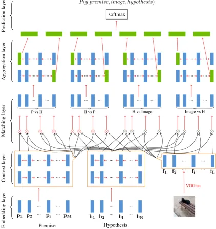
Figure 2: Vision-enhanced Bilateral Multi-Perspective Matching model (v-BiMPM).

Here, we report some further details of our implementation of the V-BiMPM model described in Section 4 of the main paper, based on the work of Wang et al. (2017). Our model is displayed in Figure 2. The core part of the original BiMPM is the matching layer. Given two d-dimensional vectors vP andvH, each replicatedl times (lis the number of ‘perspectives’) and a trainablel×dweight matrix

W, matching involves a cosine similarity computation that yields anl-dimensional matching vectorm, whose elements are defined as follows:

mk =cosine(Wk◦vP, Wk◦vH) (1)

The matching operations included are the following:

2. max-pooling, where each forward/backward contextual embedding of one sentence is compared to the embeddings of the other, retaining the maximum value for each dimension;

3. attentive matching, where first, the pairwise cosine similarity between forward/backward embed-dings of P and H is estimated, before calculating an attentive vector over the weighted sum of contextual embeddings for H and matching each forward/backward embedding of P against the attentive vector;

4. max-attentive matching, a version of attentive matching where the contextual embedding with the highest cosine is used as the attentive vector, instead of the weighted sum.

The visually-augmented version of the original model, V-BiMPM, is displayed in Figure 2. To perform multimodal matching, the visual and textual vectors are mapped to a mutual space using the following affine transformation:

vi =Wtfi+bt;fi∈Re;Wt∈Re×d;bt, vi ∈Rd (2)

whereWt,bt,fi, andvi are the weight matrix, the bias, the input features and output features, respec-tively, andtis any text (P or H). Given weight matricesW ∈ _Rl×d _{for text andU}l×d_{for images, we} compute the matching vectormbetween a textual vectorvtand image vectorvias:

mk=cosine(Wk◦vt, Uk◦vi) (3)

References

Eneko Agirre, Oier Lopez de Lacalle, and Aitor Soroa. 2017. Evaluating Multimodal Representations on Sentence Similarity : vSTS , Visual Semantic Textual Similarity Dataset. In Proceedings of the Second Workshop on Closing the Loop Between Vision and Language (ICCV’17).

Peter Anderson, Xiaodong He, Chris Buehler, Damien Teney, Mark Johnson, Stephen Gould, and Lei Zhang. 2017. Bottom-up and top-down attention for image captioning and visual question answering. arXiv preprint arXiv:1707.07998.

Mark Andrews, Gabriella Vigliocco, and David Vinson. 2009. Integrating experiential and distributional data to learn semantic representations.Psychological Review, 116(3):463–498.

Stanislaw Antol, Aishwarya Agrawal, Jiasen Lu, Margaret Mitchell, Dhruv Batra, C. Lawrence Zitnick, and Devi Parikh. 2015. VQA: Visual question answering. InInternational Conference on Computer Vision (ICCV).

Lawrence W. Barsalou. 2010. Grounded Cognition: Past, Present, and Future. Topics in Cognitive Science, 2(4):716–724.

Samuel R. Bowman, Gabor Angeli, Christopher Potts, and Christopher D. Manning. 2015. A large annotated corpus for learning natural language inference. InProceedings of the 2015 Conference on Empirical Methods in Natural Language Processing (EMNLP). Association for Computational Linguistics.

Robin Cooper, Dick Crouch, Jan Van Eijck, Chris Fox, Johan Van Genabith, Jan Jaspars, Hans Kamp, David Milward, Manfred Pinkal, Massimo Poesio, and Steve Pulman. 1996. Using the framework. Technical Report Technical Report LRE 62-051 D-16, The FraCaS Consortium.

Abhishek Das, Satwik Kottur, Khushi Gupta, Avi Singh, Deshraj Yadav, Jos´e M.F. Moura, Devi Parikh, and Dhruv Batra. 2017. Visual Dialog. InProceedings of the IEEE Conference on Computer Vision and Pattern Recognition (CVPR).

D. Giampiccolo, H. T. Dang, M. Bernardo, I. Dagan, and E. Cabrio. 2008. The fourth pascal recognising textual entailment challenge. InProceedings of the TAC 2008 Workshop on Textual Entailment.

Ross Girshick. 2015. Fast r-cnn.arXiv preprint arXiv:1504.08083.

Suchin Gururangan, Swabha Swayamdipta, Omer Levy, Roy Schwartz, Samuel R. Bowman, and Noah A. Smith. 2018. Annotation Artifacts in Natural Language Inference Data.arXiv preprint arXiv:1803.02324.

Dan Han, Pascual Martinez Gomez, and Koji Mineshima. 2017. Visual denotations for recognizing textual entail-ment. InEMNLP.

Kaiming He, Xiangyu Zhang, Shaoqing Ren, and Jian Sun. 2016. Deep residual learning for image recognition. InProceedings of the IEEE conference on computer vision and pattern recognition, pages 770–778.

Sepp Hochreiter and J¨urgen Schmidhuber. 1997. Long short-term memory. Neural computation, 9(8):1735–1780.

Micah Hodosh, Peter Young, and Julia Hockenmaier. 2013. Framing image description as a ranking task: Data, models and evaluation metrics. Journal of Artificial Intelligence Research, 47:853–899.

Justin Johnson, Bharath Hariharan, Laurens van der Maaten, Li Fei-Fei, C. Lawrence Zitnick, and Ross Girshick. 2017. Clevr: A diagnostic dataset for compositional language and elementary visual reasoning. InProceedings of CVPR 2017.

Diederik P Kingma and Jimmy Ba. 2014. Adam: A method for stochastic optimization. arXiv preprint arXiv:1412.6980.

Vladyslav Kolesnyk, Tim Rockt¨aschel, and Sebastian Riedel. 2016. Generating Natural Language Inference Chains. arXiv preprint arXiv:1606.01404.

Ranjay Krishna, Yuke Zhu, Oliver GrothJustin, Johnson Kenji Hata, Joshua Kravitz, Stephanie Chen, Yannis Kalantidis, Li-Jia Li, David A. Shamma, Michael S. Bernstein, and Li Fei-Fei. 2017. Visual genome: Con-necting language and vision using crowdsourced dense image annotations. International Journal of Computer Vision, 123(1):32–73.

Alice Lai and Julia Hockenmaier. 2017. Learning to predict denotational probabilities for modeling entailment. In

Proceedings of the 15th Conference of the European Chapter of the Association for Computational Linguistics: Volume 1, Long Papers, pages 721–730, Valencia, Spain, April. Association for Computational Linguistics.

M. Malinowski and M. Fritz. 2014. A multi-world approach to question answering about real-world scenes based on uncertain input. InAdvances in Neural Information Processing Systems.

Mitchell P Marcus, Beatrice Santorini, and Mary Ann Marcinkiewicz. 1993. Building a large annotated corpus of English: The Penn Treebank.Computational Linguistics, 19(2):313–330.

Marco Marelli, Stefano Menini, Marco Baroni, Luisa Bentivogli, Raffaella Bernardi, and Roberto Zamparelli. 2014. A sick cure for the evaluation of compositional distributional semantic models. InProceedings of LREC 2014, pages 216–223. ELRA.

George A. Miller. 1995. WordNet: a lexical database for English.Communications of the ACM, 38(11):39–41.

M. Mironenco, D. Kianfar, K. Tran, E. Kanoulas, and E. Gavves. 2017. Examining cooperation in visual di-alog models. In Neural Informations Processing Systems, Workshop on Visually-Grounded Interaction and Language.

Vinod Nair and Geoffrey E Hinton. 2010. Rectified linear units improve restricted boltzmann machines. In

Proceedings of the 27th international conference on machine learning (ICML-10), pages 807–814.

Nikita Nangia, Adina Williams, Angeliki Lazaridou, and Samuel R Bowman. 2017. The RepEval 2017 Shared Task: Multi-Genre Natural Language Inference with Sentence Representations. arXiv preprint arXiv:1707.08172.

R. Passonneau, N. Habash, and O. Rambow. 2006. Inter-annotator agreement on a multilingual semantic anno-tation task. In Proceedings of the International Conference on Language Resources and Evaluation (LREC), pages 1951–1956.

Jeffrey Pennington, Richard Socher, and Christopher D Manning. 2014. GloVe: Global Vectors for Word Rep-resentation. In Proceedings of the 2014 Conference on Empirical Methods in Natural Language Processing (EMNLP’14), pages 1532–1543, Doha, Qatar. Association for Computational Linguistics.

Karen Simonyan and Andrew Zisserman. 2014. Very deep convolutional networks for large-scale image recogni-tion. arXiv preprint arXiv:1409.1556.

Vincent Sitzmann, Martina Marek, and Leonid Keselman. 2016. Multimodal natural language inference. Techni-cal report, Standford.

Nitish Srivastava, Geoffrey Hinton, Alex Krizhevsky, Ilya Sutskever, and Ruslan Salakhutdinov. 2014. Dropout: A simple way to prevent neural networks from overfitting. The Journal of Machine Learning Research, 15(1):1929–1958.

Janez Starc and Dunja Mladeni´c. 2017. Constructing a Natural Language Inference dataset using generative neural networks. Computer Speech and Language, 46:94–112.

Alane Suhr, Mike Lewis, James Yeh, and Yoav Artzi. 2017. A corpus of natural language for visual reasoning. InProceedings of the 55th Annual Meeting of the Association for Computational Linguistics (Volume 2: Short Papers), pages 217–223, Vancouver, Canada, July. Association for Computational Linguistics.

Ming Tan, Cicero dos Santos, Bing Xiang, and Bowen Zhou. 2016. LSTM-based Deep Learning Models for Non-factoid Answer Selection. arXiv preprint arXiv:1511.04108, pages 1–11.

Damien Teney, Peter Anderson, Xiaodong He, and Anton van den Hengel. 2017. Tips and tricks for visual question answering: Learnings from the 2017 challenge. arXiv preprint arXiv:1708.02711.

Ivan Vendrov, Ryan Kiors, Sanja Fidler, and Raquel Urtasun. 2016. Order-embeddings of images and language. InProceedings of the International Conference of Learning Representations (ICLR).

Zhiguo Wang, Wael Hamza, and Radu Florian. 2017. Bilateral Multi-Perspective Matching for Natural Lan-guage Sentences. InProceedings of the Twenty-Sixth International Joint Conference on Artificial Intelligence (IJCAI’17), pages 4144–4150, Melbourne.

Adina Williams, Nikita Nangia, and Samuel R. Bowman. 2018. A Broad-Coverage Challenge Corpus for Sentence Understanding through Inference. InProceedings of NAACL.

K. Xu, J. L. Ba, R. Kiros, K. Cho, A. Courville, R. Salakhutdinov, R. Zemel, and Y. Bengio. 2015. Show, attend and tell: Neural image caption generation with visual attention. InProceedings of the International Conference on Machine Learning (ICML).