YNU HPCC at IJCNLP 2017 Task 1: Chinese Grammatical Error Diagnosis Using a Bi directional LSTM CRF Model

YNU-HPCC at IJCNLP-2017 Task 1: Chinese Grammatical Error

Diagnosis Using a Bi-directional LSTM-CRF Model

Quanlei Liao, Jin Wang, Jinnan Yang and Xuejie Zhang

School of Information Science and Engineering Yunnan University

Kunming, P.R. China

Contact:[email protected]

Abstract

Building a system to detect Chinese gram-matical errors is a challenge for natural-language processing researchers. As Chi-nese learners are increasing, developing such a system can help them study Chinese more easily. This paper introduces a bi-directional long short-term memory (BiL-STM) - conditional random field (CRF) model to produce the sequences that in-dicate an error type for every position of a sentence, since we regard Chinese grammatical error diagnosis (CGED) as a sequence-labeling problem. Among the participants this year of CGED shard task, our model ranked third in the detection-level and identification-detection-level results. In the position-level, our results ranked second a-mong the participants.

1 Introduction

With China’s rapid development, more and more foreign people have begun to learn Chinese. Writ-ing is an important part of language learnWrit-ing, and grammar is the basis of writing. Traditional learn-ing methods rely on artificial work to point out grammatical errors in an article. This requires more time and labor costs. Thus, it is quite practi-cal to develop a system that can automatipracti-cally cor-rect the grammatical errors in an article. This is the aim of the CGED shared task.

In the shared task, Chinese-grammar errors are divided into four types: redundant words, word-selection errors, missing words, and incorrec-t word order (Lee et al.,2016). They are represent-ed as uppercase letters “R”, “S”, “M”, and “W”, respectively. For each sentence, the task should first determine whether the sentence is correct. If

the sentence is incorrect, it should indicate the spe-cific error types and their locations.

In this paper, the CGED task is treated as a se-quence labeling problem, which is a classic natural language processing problem. The traditional so-lutions are a series of statistical learning methods, including the hidden Markov model (HMM), the maximum-entropy Markov model (MEMM), and the conditional random field.

The HMM model makes two assumptions. First, that the current implicit state is only related to the last implied state; second, that the current output state is only related to the current implied state (Dugad and Desai,1996). However, the real-ity is not so simple. A CRF uses the entire output sequence and two adjacent implicit states to find a conditional probability (Lafferty et al., 2001). It can fit more complex situations. Practice has proven that the CRF works better than other mod-els.

Recently, artificial neural networks have been used to do natural language processing tasks. For the sequence labeling problem, because of its e-qual length output, a recurrent neural network (RNN) is an appropriate model. It is more capable of understanding the information context; howev-er, this is not a good method for learning state transfer laws. To improve the problems of explod-ing and vanishexplod-ing gradients, new RNN units, e.g., long short-term memory (LSTM) and gated recur-rent units (GRUs) (Chung et al.,2014), have been proposed.

In this study, we propose a BiLSTM-CRF mod-el. Our model combines statistical learning with neural networks. The BiLSTM is used to obtain information about long or short distances in two directions (Huang et al.,2015). It then feeds the information to the CRF. Thus, the CRF can better use conditional probabilities to fit the data without handmade features. The CRF and LSTM models

are also used as part of the experiment to compare the models’ performance.

The rest of this paper is organized as follows. Section 2 describes our model in detail. Section 3 presents our experiment, including the data pre-processing and results. Conclusions are drawn in Section 4.

2 Proposed Model

The proposed model consists of three major parts: the word-embedding layer, the bi-directional LST-M layer, and the CRF layer. CRF is a traditional s-tatistical learning method for sequence labeling. It has two limits. First, it heavily depends on hand-crafted features. Second, it cannot capture long distance context information. The context infor-mation for a CGED task is very important. For example, here are two correct sentences.

• “只有努力，才_能过_{的更好。” (Only you}

work hard, you can be better.)

• “只要努力，就_能过_{的更好。” (As long as}

you work hard, you will be able to be better.)

It is impossible to determine whether the sentence, “才_能过的_更好_。” is correct without the previous

context information. On the other hand, handcraft-ed features greatly increase the workload. Thus, our model combines an RNN with a CRF to im-prove the above problems. To capture informa-tion from two direcinforma-tions (Ma and Hovy,2016), we use a bi-directional RNN instead of a unidirection-al RNN. In addition, an LSTM cell is selected to avoid vanishing and exploding gradients ( Sunder-meyer et al.,2012).

We trained four models for four error types be-cause there may be two or more errors in one posi-tion. Each model is given the original text index as input, its label sequence outputs 0 for correct and 1 for error.

The model includes three layers: a word-embedding layer to transfer the word index into word embedding, a BiLSTM layer to extract the information and features for each position, and a CRF layer to decode and produce labels. The three layers are introduced in the following sections.

2.1 Embedding Layer

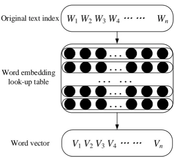
A diagram of the embedding layer’s structure is shown in Figure 1. It shows a pre-trained word-embedding lookup table. Every line of this table

W1 W2 W3 W4 Wn

V1 V2 V3 V4 Vn

... ...

... ... ... ... Original text index

Word embedding look-up table

Word vector

Figure 1: Embedding Layer

stands for one Chinese word. Therefore, the orig-inal text of the training data should be turned into a sequence of indexes for every word. This lay-er takes a sequence that contains the word indices, e.g., w1, w2,. . . , wi,. . . , wn where wi, is an in-dex number indicating the position of the original word in the table. Then, the layer finds the word vector for every index and outputs them in a new sequence, e.g.,v1,v2,. . . ,vi,. . . ,vnwherevi is a

word vector.

If the dimensionality of the original text index is Nand the dimensionality of the word vector isM, the dimensionality of the output sequence should beM ∗N.

2.2 Bi-directional LSTM Layer

An RNN can effectively extract features from the entire sentence because of its ability to capture context information. For the reasons mentioned above, a bi-directional LSTM network was cho-sen.

An LSTM is a special type of RNN unit that can learn long-term dependency information. It is designed to avoid the long-term dependence prob-lem. An LSTM can remove or increase the infor-mation to a cell state using a well-designed struc-ture called a “gate”. The gate determines whether information should pass. The LSTM uses the following formulas (Hochreiter and Schmidhuber, 1997):

it=σ(Wvivt+Whiht−1+bi) (1)

V3

V1 V2 V4

Forward LSTM

Backward LSTM

Output X1

LSTM

LSTM LSTM LSTM

X2 X3 X4 LSTM LSTM

LSTM LSTM

Figure 2: Bi-directional LSTM Layer

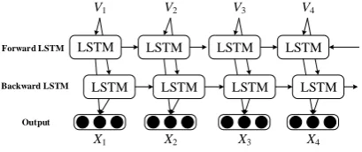
ht=ottanh(ct) (5) where v is the input vector from the embedding layer.σis the sigmoid activation function. iis the input gate, f is the forget gate, ando is the out-put gate. Parameters{Wvi,Whi,Wvf,Whf,Wvc, Whc, Wvo, Who, bi, bf, bc, bo} are the weights and biases of an LSTM cell. c is the cell vector andhis the hidden cell. K represents the output dimensionality of the LSTM unit.N is the dimen-sionality of the word vector. The size of the last four bias vectors areKand the others areN∗K. Figure 2 shows a bi-directional LSTM network. The embedding output is fed into two LSTM lay-ers with forward and backward directions. Two outputs from two layers at one position are linked into a new vector as the layer’s output.

The dimensionality of the input is M ∗N. M is the length of the original text. Each word vec-tor of input is also called an RNN time step. For instance, v1, v2,. . . , vi,. . . , vn is input, each vi

is a time step. For each time step, vi is fed into two LSTMs; the forward LSTM layer produces an output vector oi−forward with dimensionali-ty K, and the backward LSTM layer produces oi−backward. Therefore, the result of a time step isxi(oi−forward, oi−backward)and the dimension-ality is2∗K, which is the result of combining the two layers’ output. Thus, the dimensionality of the final output isM∗(2∗K).

2.3 CRF Layer

Because of the importance of the relationships be-tween neighboring tags in CGED, a CRF is select-ed to capture the relationship. The CRF is a type of undirected discriminative graph model. In general, a CRF is a Markov random field with an observa-tion set. A general CRF is defined as a Markov random field with random variable Y under the condition of random variableX. Y constitutes a Markov random field represented by an undirected graph, as in the formula below (Sutton and

Mccal-X1 X2 X3 Xn

Input

Y1 Y2 Y3 Yn

CRF Layer

Figure 3: CRF Layer lum,2010):

P(Yv|X, Yw, w6=v)=P(Yv|X, Yw, w∼v) (6) where operator∼means thatwandvhave a pub-lic edge.Xis the input variable or state sequence, andY is the output variable or tag sequence. In our problem, we assume that X andY have the same linear structure, as shown in Figure 3.

The conditional probability of random variable ywith valuexis given as follows:

P(y|x) = n

Q

i=1Mi(yi−1, yi, x)

Z(x) (7) The denominator is a normalization item:

Z(x) =X y

n

Y

i=1

Mi(yi−1, yi, x) (8)

whereMi(y0, y00, x)is a potential function,xis the input vector produced by the BiLSTM layer andy is the labeling of the input sentence.

3 Experiment

This section describes the contents of the ex-periment, including the training data processing, choice of parameters, experimental results, etc.

3.1 Dataset

The word embedding was trained using the word2vec toolkit with the Chinese Wikipedia cor-pus. According to the experimental results, the word-embedding results from word2vec are bet-ter than GloVe (Yang et al.,2016). In addition to the CGED17 training data, the HSK (i.e., Chinese Proficiency Test) training data from CGED16 was used. The number of training sets is 20,048, with 10,447 from CGED17 and 9,601 from CGED16.

Model Acc Pre Rec F1 CRF 0.1805 0.1136 0.1483 0.1287 LSTM 0.1696 0.1824 0.0816 0.1128 BiLSTM-CRF 0.3325 0.2769 0.3502 0.3093

Table 1: Comparative results of three models.

3.2 Implementation Details

The experiment contains three models for compar-ison: CRF, LSTM, and BiLSTM-CRF. CRF rep-resents the statistical learning method, which is the best simple statistical learning model in a vari-ety of sequence labeling tasks. LSTM is a typical neural network model for sequence labeling. The above two models were used as the baseline for the experiment. The last model, proposed in this pa-per, combines both neural network and statistical learning models.

The CRF model was implemented using the CRF++ toolkit. CRF++ is an open-source, easy-to-use implementation of CRF, written in C++. The LSTM model and the BiLSTM-CRF mod-el were implemented using the Keras framework with a Tensorflow backend. The CRF layer im-plementation in the BiLSTM-CRF model used K-eras contrib.

The training data for the three models comes from CGED16 or CGED17. Hence, the training data is regarded as a hyper-parameter. It will be CGED16 or CGED17 or a combination of both. In addition, there is a public hyper-parameter for the three models. The hyper-parameter for the CR-F model is c, which controls the over-fitting of the training data. The hyper-parameters for LSTM and BiLSTM-CRF include the LSTM cell number and the training epoch.

Some empirical parameters are given as candi-date values for the model. A grid search algorithm was used to find the best hyper-parameter combi-nations.

To evaluate the model’s performance, we used four metrics such as accuracy (Acc), precision (Pre), recall (Rec) and F1-score (F1) for all three models on CGED16 HSK test data. Table 1 shows the best results for each model on position-level. The results show that the BiLSTM-CRF model has the best results in Table 1.

3.3 Experimental Results

Five teams submitted 13 results. We submit-ted three running results. The three results were produced by the three BiLSTM-CRF models that

Parameter Dataset LSTM cell Epoch

Run1 CGED16,17 120 22

Run2 CGED16,17 100 18

Run3 CGED16 100 18

Table 2: Parameter selection for BiLSTM-CRF models.

Results _Acc Detection-Level_{Pre Rec F1} Run1 0.5796 0.65 0.7163 0.6816 Run2 0.5891 0.6417 0.7829 0.7053 Run3 0.5311 0.6298 0.6148 0.6222

Table 3: Comparative results on detection-level.

had the best three results on the CGED16 HSK test data. The three results have different hyper-parameters, as shown in Table 2.

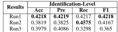
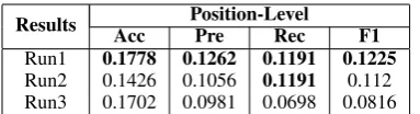
The next three tables show the final test result-s for the three BiLSTM-CRF modelresult-s. Table 3 shows the detection-level results. Table 4 shows the identification-level results. Table 5 shows the position-level results.

The false positive (FP) rates of the three results of BiLSTM-CRF models are 0.5796, 0.7383, and 0.614 shown in Table 6. The highest one is over 70%. This is because the model uses four sub-models to generate the sentence label. If only one model misjudges the label of one position, from 0 to 1, it will produce a false negative (FN) sam-ple. Thus, the model produces a high false positive rate. In addition, the experimental results show that the recall of the first two results is better than the previous in the detection level. This model is more likely to produce positive examples.

4 Conclusion

Compared with most previous models (Lee et al., 2016), the F1-score of the position level greatly increased with the CGED16 HSK test data. It was observed that neural network and statistical-learning methods could be combined to obtain better results. Among the participants this year, our model ranked third in the detection-level and identification-level results. In the position-level,

Results _Acc Identification-Level_{Pre Rec F1} Run1 0.4218 0.4219 0.4217 0.4218 Run2 0.3819 0.3825 0.4575 0.4167 Run3 0.3979 0.4086 0.3298 0.365

Results _Acc Position-Level_{Pre Rec F1} Run1 0.1778 0.1262 0.1191 0.1225 Run2 0.1426 0.1056 0.1191 0.112 Run3 0.1702 0.0981 0.0698 0.0816

Table 5: Comparative results on position-Level.

Result False Positive Rate

Run1 0.5796

Run2 0.7383

Run3 0.614

Table 6: False positive rates of three results.

our results ranked second among the participants. Our model is a combination of BiLSTM and CRF. It combines the extraction capabilities of the LSTM context information and the condition-al probability of CRF’s loccondition-al features. More com-plex models contain more parameters that need to be trained. Thus, more training data can improve the model; too little training data may cause over-fitting.

The shared task provided us with more in-depth understanding about CGED. Our next step is to obtain more training data to enhance the model.

Acknowledgments

This work was supported by the National Natural Science Foundation of China (NSFC) under Grant No.61702443 and No.61762091, and in part by Educational Commission of Yunnan Province of China under Grant No.2017ZZX030.The authors would like to thank the anonymous reviewers and the area chairs for their constructive comments.

References

Junyoung Chung, Caglar Gulcehre, KyungHyun Cho, and Yoshua Bengio. 2014. Empirical evaluation of gated recurrent neural networks on sequence model-ing. InarXiv preprint arXiv:1412.3555.

Rakesh Dugad and U B Desai. 1996. A tutorial on hid-den markov models. In Proceedings of the IEEE, pages 257–286.

Sepp Hochreiter and J¨urgen Schmidhuber. 1997. Long short-term memory. Neural Computation, 9(8):1735–1780.

Zhiheng Huang, Wei Xu, and Kai Yu. 2015. Bidirec-tional lstm-crf models for sequence tagging. In arX-iv preprint arXarX-iv:1508.01991.

John Lafferty, Andrew Mccallum, and Fernando Pereira. 2001. Conditional random fields:

Prob-abilistic models for segmenting and labeling se-quence data. In Proceedings of the International Conference on Machine Learning (ICML-01), pages 282–289.

Lung-Hao Lee, Liang-Chih Yu, and Li-Ping Chang. 2016. Overview of nlp-tea 2016 shared task for Chi-nese grammatical error diagnosis. In Proceedings of the 3rd Workshop on Natural Language Process-ing Techniques for Educational Applications (NLP-TEA-16), pages 40–48.

Xuezhe Ma and Eduard Hovy. 2016. End-to-end se-quence labeling via bi-directional lstm-cnns-crf. In

Proceedings of the 54th Annual Meeting of the As-sociation for Computational Linguistics (ACL-16), pages 1064–1074.

Martin Sundermeyer, Ralf Schluter, and Hermann Ney. 2012. Lstm neural networks for language modeling. InProceedings of INTERSPEECH 2013, pages 601– 608.

Charles Sutton and Andrew Mccallum. 2010.An Intro-duction to Conditional Random Fields. Now Pub-lishers Inc.