Constituent Parsing by Classification

Constituent Parsing by Classification

Joseph Turian and I. Dan Melamed

{lastname}@cs.nyu.edu

Computer Science Department New York University New York, New York 10003

Abstract

Ordinary classification techniques can drive a conceptually simple constituent parser that achieves near state-of-the-art accuracy on standard test sets. Here we present such a parser, which avoids some of the limitations of other discriminative parsers. In particular, it does not place any restrictions upon which types of fea-tures are allowed. We also present sev-eral innovations for faster training of dis-criminative parsers: we show how train-ing can be parallelized, how examples can be generated prior to training with-out a working parser, and how indepen-dently trained sub-classifiers that have

never done any parsing can be effectively

combined into a working parser. Finally, we propose a new figure-of-merit for best-first parsing with confidence-rated infer-ences. Our implementation is freely

avail-able at:http://cs.nyu.edu/˜turian/

software/parser/

1 Introduction

Discriminative machine learning methods have im-proved accuracy on many NLP tasks, such as POS-tagging (Toutanova et al., 2003), machine translation (Och & Ney, 2002), and relation extraction (Zhao & Grishman, 2005). There are strong reasons to believe the same would be true of parsing. However, only limited advances have been made thus far, perhaps

due to various limitations of extant discriminative parsers. In this paper, we present some innovations aimed at reducing or eliminating some of these lim-itations, specifically for the task of constituent pars-ing:

• We show how constituent parsing can be

per-formed using standard classification techniques.

• Classifiers for different non-terminal labels can be

induced independently and hence training can be parallelized.

• The parser can use arbitrary information to

evalu-ate candidevalu-ate constituency inferences.

• Arbitrary confidence scores can be aggregated in

a principled manner, which allows beam search. In Section 2 we describe our approach to parsing. In Section 3 we present experimental results.

The following terms will help to explain our work. A span is a range over contiguous words in the in-put sentence. Spans cross if they overlap but nei-ther contains the onei-ther. An item (or constituent) is a (span,label) pair. A state is a set of parse items, none of which may cross. A parse inference is a pair (S,i), given by the current state S and an item i to be added to it. A parse path (or history) is a sequence of parse inferences over some input sentence (Klein & Manning, 2001). An item ordering (ordering, for short) constrains the order in which items may be in-ferred. In particular, if we prescribe a complete item ordering, the parser is deterministic (Marcus, 1980) and each state corresponds to a unique parse path. For some input sentence and gold-standard parse, a state is correct if the parser can infer zero or more additional items to obtain the gold-standard parse. A parse path is correct if it leads to a correct state. An

inference is correct if adding its item to its state is correct.

2 Parsing by Classification

Recall that with typical probabilistic parsers, our goal is to output the parse ˆP with the highest like-lihood for the given input sentence x:

ˆ

P=arg max

P∈P(x)

Pr(P) (1)

=arg max

P∈P(x)

Y

I∈P

Pr(I) (2)

or, equivalently,

=arg max

P∈P(x)

X

I∈P

log(Pr(I)) (3)

where each I is a constituency inference in the parse path P.

In this work, we explore a generalization in which each inference I is assigned a real-valued confidence score Q(I) and individual confidences are

aggre-gated using some function A, which need not be a

sum or product: ˆ

P=arg max

P∈P(x)

A

I∈PQ(I) (4)

In Section 2.1 we describe how we induce scoring function Q(I). In Section 2.2 we discuss the

aggre-gation function A. In Section 2.3 we describe the

method used to restrict the size of the search space over P(x).

2.1 Learning the Scoring Function Q(I)

During training, our goal is to induce the scoring function Q, which assigns a real-valued confidence score Q(I) to each candidate inference I (Equa-tion 4). We treat this as a classifica(Equa-tion task: If infer-ence I is correct, we would like Q(I) to be a positive value, and if inference I is incorrect, we would like Q(I) to be a negative value.

Training discriminative parsers can be computa-tionally very expensive. Instead of having a single classifier score every inference, we parallelize train-ing by inductrain-ing 26 sub-classifiers, one for each

con-stituent labelλin the Penn Treebank (Taylor,

Mar-cus, & Santorini, 2003): Q(Iλ) = Qλ(Iλ), where Qλ is the λ-classifier and Iλ is an inference that in-fers a constituent with labelλ. For example, theVP

-classifier QVPwould score the VP-inference in

Fig-ure 1, preferably assigning it a positive confidence.

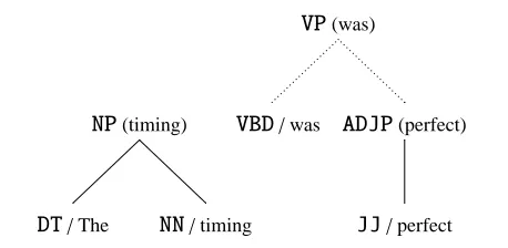
Figure 1 A candidate VP-inference, with head-children annotated using the rules given in (Collins, 1999).

VP(was)

NP(timing) VBD/was ADJP(perfect)

DT/The NN/timing JJ/perfect

Eachλ-classifier is independently trained on training set Eλ, where each example eλ ∈Eλis a tuple (Iλ,y), Iλis a candidateλ-inference, and y∈ {±1}. y= +1 if Iλis a correct inference and−1 otherwise. This

ap-proach differs from that of Yamada and Matsumoto

(2003) and Sagae and Lavie (2005), who parallelize according to the POS tag of one of the child items.

2.1.1 Generating Training Examples

Our method of generating training examples does not require a working parser, and can be run prior to any training. It is similar to the method used in the literature by deterministic parsers (Yamada & Mat-sumoto, 2003; Sagae & Lavie, 2005) with one ex-ception: Depending upon the order constituents are inferred, there may be multiple bottom-up paths that lead to the same final parse, so to generate training examples we choose a single random path that leads

to the gold-standard parse tree.1 The training

ex-amples correspond to all candidate inferences con-sidered in every state along this path, nearly all of

which are incorrect inferences (with y = −1). For

instance, only 4.4% of candidateNP-inferences are

correct.

2.1.2 Training Algorithm

During training, for each labelλwe induce

scor-ing function Qλ to minimize the loss over training

examples Eλ:

Qλ=arg min

Q0

λ

X

(Iλ,y)∈Eλ

L(y·Q0_λ(Iλ)) (5)

1 _{The particular training tree paths used in our experiments are}

where y· Qλ(Iλ) is the margin of example (Iλ,y). Hence, the learning task is to maximize the margins of the training examples, i.e. induce scoring function Qλsuch that it classifies correct inferences with pos-itive confidence and incorrect inferences with nega-tive confidence. In our work, we minimized the lo-gistic loss:

L(z)=log(1+exp(−z)) (6)

i.e. the negative log-likelihood of the training sam-ple.

Our classifiers are ensembles of decisions trees, which we boost (Schapire & Singer, 1999) to min-imize the above loss using the update equations given in Collins, Schapire, and Singer (2002). More specifically, classifier QT_λ is an ensemble comprising decision trees q1_λ, . . . ,qT_λ, where:

QT_λ(Iλ)= T

X

t=1

qt_λ(Iλ) (7)

At iteration t, decision tree qt_λ is grown, its leaves are confidence-rated, and it is added to the ensemble. The classifier for each constituent label is trained

in-dependently, so we henceforth omitλsubscripts.

An example (I,y) is assigned weight wt(I,y):2

wt(I,y)= 1

1+exp(y·Qt−1_(I)) (8)

The total weight of y-value examples that fall in leaf f is Wt

f,y:

Wt_f,y = X

(I,y0_)∈E

y0_=y,I∈f

wt(I,y) (9)

and this leaf has loss Zt_f:

Zt_f =2· qW_ft_,+·Wt_f,− (10)

Growing the decision tree: The loss of the entire decision tree qt is

Z(qt)= X

leaf f∈qt

Zt_f (11)

2 _{If we were to replace this equation with w}t_{(I,y) =} exp(y·Qt−1_(I))−1_{, but leave the remainder of the algorithm}

un-changed, this algorithm would be confidence-rated AdaBoost (Schapire & Singer, 1999), minimizing the exponential loss

L(z) = exp(−z). In preliminary experiments, however, we

found that the logistic loss provided superior generalization accuracy.

We will use Ztas a shorthand for Z(qt). When grow-ing the decision tree, we greedily choose node splits to minimize this Z (Kearns & Mansour, 1999). In particular, the loss reduction of splitting leaf f us-ing featureφinto two children, f∧φand f∧ ¬φ, is

∆Zt f(φ):

∆Zt_f(φ)=Zt_f −(Zt_f∧φ+Zt_f∧¬φ) (12)

To split node f , we choose the ˆφ that reduces loss

the most:

ˆ

φ=arg max

φ∈Φ

∆Zt_f(φ) (13)

Confidence-rating the leaves: Each leaf f is confidence-rated asκt_f:

κt_f = 1

2·log

Wt_f,++

Wt f,−+

(14)

Equation 14 is smoothed by the term (Schapire

& Singer, 1999) to prevent numerical instability in the case that either Wt_f,+ or Wt_f,− is 0. In our

ex-periments, we used = 10−8. Although our

exam-ple weights are unnormalized, so far we’ve found

no benefit from scalingas Collins and Koo (2005)

suggest. All inferences that fall in a particular leaf node are assigned the same confidence: if inference I falls in leaf node f in the tth decision tree, then qt(I)=κt_f.

2.1.3 Calibrating the Sub-Classifiers

An important concern is when to stop growing the decision tree. We propose the minimum reduction in loss (MRL) stopping criterion: During training,

there is a valueΘt at iteration t which serves as a

threshold on the minimum reduction in loss for leaf splits. If there is no splitting feature for leaf f that reduces loss by at leastΘt then f is not split. For-mally, leaf f will not be bisected during iteration t if maxφ∈Φ∆Zt_f(φ) < Θt. The MRL stopping criterion is essentially`₀regularization:Θtcorresponds to the

`0penalty parameter and each feature with non-zero

confidence incurs a penalty ofΘt, so to outweigh the penalty each split must reduce loss by at leastΘt.

Θt decreases monotonically during training at

the slowest rate possible that still allows

train-ing to proceed. We start by initializtrain-ing Θ1 to ∞,

and at the beginning of iteration t we decreaseΘt

only if the root node ∅ of the decision tree

Θt = min(Θt−1,maxφ∈Φ∆Z_∅t(φ)). In this manner, the decision trees are induced in order of decreasingΘt.

During training, the constituent classifiers Qλ

never do any parsing per se, and they train at dif-ferent rates: If λ , λ0, then Θt_λ isn’t necessarily equal toΘt

λ0. We calibrate the different classifiers by

picking some meta-parameter ˆΘ and insisting that

the sub-classifiers comprised by a particular parser have all reached some fixedΘin training. Given ˆΘ, the constituent classifier for label λ is Qt_λ, where

Θt_λ ≥ Θˆ > Θt_λ+1. To obtain the final parser, we cross-validate ˆΘ, picking the value whose set of con-stituent classifiers maximizes accuracy on a devel-opment set.

2.1.4 Types of Features used by the Scoring Function

Our parser operates bottom-up. Let the frontier of a state be the top-most items (i.e. the items with no parents). The children of a candidate inference are those frontier items below the item to be inferred, the left context items are those frontier items to the left of the children, and the right context items are those frontier items to the right of the children. For exam-ple, in the candidateVP-inference shown in Figure 1,

the frontier comprises theNP,VBD, andADJPitems,

theVBDandADJPitems are the children of theVP

-inference (theVBDis its head child), theNPis the left context item, and there are no right context items.

The design of some parsers in the literature re-stricts the kinds of features that can be usefully and efficiently evaluated. Our scoring function and pars-ing algorithm have no such limitations. Q can, in principle, use arbitrary information from the history to evaluate constituent inferences. Although some of our feature types are based on prior work (Collins, 1999; Klein & Manning, 2003; Bikel, 2004), we note that our scoring function uses more history in-formation than typical parsers.

All features check whether an item has some property; specifically, whether the item’s la-bel/headtag/headword is a certain value. These fea-tures perform binary tests on the state directly, un-like Henderson (2003) which works with an inter-mediate representation of the history. In our baseline setup, feature setΦ contained five different feature types, described in Table 1.

Table 2 Feature item groups.

• all children

• all non-head children

• all non-leftmost children

• all non-rightmost children

• all children left of the head • all children right of the head

• head-child and all children left of the head

• head-child and all children right of the head

2.2 Aggregating Confidences

To get the cumulative score of a parse path P, we

ap-ply aggregatorAover the confidences Q(I) in

Equa-tion 4. Initially, we definedAin the customary fash-ion as summing the loss of each inference’s confi-dence:

ˆ

P=arg max

P∈P(x)

      −

X

I∈P

L (Q(I))

     

 (15)

with the logistic loss L as defined in Equation 6. (We negate the final sum because we want to minimize

the loss.) This definition ofAis motivated by

view-ing L as a negative log-likelihood given by a logistic function (Collins et al., 2002), and then using Equa-tion 3. It is also inspired by the multiclass loss-based decoding method of Schapire and Singer (1999). With this additive aggregator, loss monotonically in-creases as inferences are added, as in a PCFG-based parser in which all productions decrease the cumu-lative probability of the parse tree.

In preliminary experiments, this aggregator gave disappointing results: precision increased slightly, but recall dropped sharply. Exploratory data analy-sis revealed that, because each inference incurs some positive loss, the aggregator very cautiously builds the smallest trees possible, thus harming recall. We

had more success by defining A to maximize the

minimum confidence. Essentially,

ˆ

P=arg max

P∈P(x) min

I∈P Q(I) (16)

Ties are broken according to the second lowest con-fidence, then the third lowest, and so on.

2.3 Search

Table 1 Types of features.

• Child item features test if a particular child item has some property. E.g. does the item one right of the

head have headword “perfect”? (True in Figure 1)

• Context item features test if a particular context item has some property. E.g. does the first item of left

context have headtagNN? (True)

• Grandchild item features test if a particular grandchild item has some property. E.g. does the leftmost

child of the rightmost child item have labelJJ? (True)

• Exists features test if a particular group of items contains an item with some property. E.g. does some

non-head child item have labelADJP? (True) Exists features select one of the groups of items specified in

Table 2. Alternately, they can select the terminals dominated by that group. E.g. is there some terminal item dominated by non-rightmost children items that has headword “quux”? (False)

consider every possible sequence of inferences, we use beam search to restrict the size of P(x). As an additional guard against excessive computation, search stopped if more than a fixed maximum num-ber of states were popped from the agenda. As usual, search also ended if the highest-priority state in the agenda could not have a better aggregated score than the best final parse found thus far.

3 Experiments

Following Taskar, Klein, Collins, Koller, and

Man-ning (2004), we trained and tested on≤15 word

sen-tences in the English Penn Treebank (Taylor et al.,

2003), 10% of the entire treebank by word count.3

We used sections 02–21 (9753 sentences) for train-ing, section 24 (321 sentences) for development, and section 23 (603 sentences) for testing, prepro-cessed as per Table 3. We evaluated our parser us-ing the standard PARSEVAL measures (Black et al., 1991): labelled precision, recall, and F-measure (LPRC, LRCL, and LFMS, respectively), which are computed based on the number of constituents in the parser’s output that match those in the gold-standard parse. We tested whether the observed differences in

PARSEVAL measures are significant at p=0.05

us-ing a stratified shuffling test (Cohen, 1995, Section 5.3.2) with one million trials.4

As mentioned in Section 1, the parser cannot in-fer any item that crosses an item already in the state.

3 _{There was insufficient time before deadline to train on all}

sentences.

4 _{The shuffling test we used was originally implemented}

by Dan Bikel (http://www.cis.upenn.edu/˜dbikel/ software.html) and subsequently modified to compute p-values for LFMS differences.

We placed three additional candidacy restrictions on inferences: (a) Items must be inferred under the bottom-up item ordering; (b) To ensure the parser does not enter an infinite loop, no two items in a state can have both the same span and the same label;

(c) An item can have no more than K = 5 children.

(Only 0.24% of non-terminals in the preprocessed development set have more than five children.) The number of candidate inferences at each state, as well as the number of training examples generated by the algorithm in Section 2.1.1, is proportional to K. In our experiment, there were roughly|Eλ| ≈ 1.7 mil-lion training examples for each classifier.

3.1 Baseline

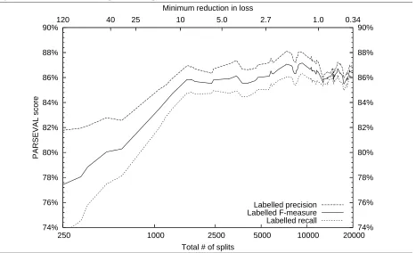
In the baseline setting, context item features (Sec-tion 2.1.4) could refer to the two nearest items of context in each direction. The parser used a beam width of 1000, and was terminated in the rare event that more than 10,000 states were popped from the agenda. Figure 2 shows the accuracy of the base-line on the development set as training progresses.

Cross-validating the choice of ˆΘagainst the LFMS

(Section 2.1.3) suggested an optimum of ˆΘ =1.42.

At this ˆΘ, there were a total of 9297 decision tree splits in the parser (summed over all constituent

classifiers), LFMS = 87.16, LRCL = 86.32, and

LPRC=88.02.

3.2 Beam Width

To determine the effect of the beam width on the

base-Table 3 Steps for preprocessing the data. Starred steps are performed only on input with tree structure. 1. * Strip functional tags and trace indices, and remove traces.

2. * ConvertPRTtoADVP. (This convention was established by Magerman (1995).)

3. Remove quotation marks (i.e. terminal items tagged‘‘or’’). (Bikel, 2004)

4. * Raise punctuation. (Bikel, 2004)

5. Remove outermost punctuation.a

6. * Remove unary projections to self (i.e. duplicate items with the same span and label). 7. POS tag the text using Ratnaparkhi (1996).

8. Lowercase headwords.

9. Replace any word observed fewer than 5 times in the (lower-cased) training sentences withUNK.

a _{As pointed out by an anonymous reviewer of Collins (2003), removing outermost punctuation may discard useful information.} It’s also worth noting that Collins and Roark (2004) saw a LFMS improvement of 0.8% over their baseline discriminative parser after adding punctuation features, one of which encoded the sentence-final punctuation.

Figure 2 PARSEVAL scores of the baseline on the≤15 words development set of the Penn Treebank. The

top x-axis shows accuracy as the minimum reduction in loss ˆΘdecreases. The bottom shows the

correspond-ing number of decision tree splits in the parser, summed over all classifiers.

74% 76% 78% 80% 82% 84% 86% 88% 90%

20000 10000

5000 2500

1000 250

74% 76% 78% 80% 82% 84% 86% 88% 90% 0.34 1.0

2.7 5.0

10 25

40 120

PARSEVAL score

Total # of splits Minimum reduction in loss

Labelled precision Labelled F-measure Labelled recall

line results on the development set with a beam

width of 1 and a beam width of 1000.5 The wider

beam seems to improve the PARSEVAL scores of the parser, although we were unable to detect a sta-tistically significant improvement in LFMS on our relatively small development set.

5 _{Using a beam width of 100,000 yielded output identical to}

using a beam width of 1000.

3.3 Context Size

Table 5 compares the baseline to parsers that could not examine as many context items. A significant portion of the baseline’s accuracy is due to contex-tual clues, as evidenced by the poor accuracy of the no context run. However, we did not detect a

signif-icant difference between using one context item or

Table 4 PARSEVAL results on the ≤ 15 words development set of the baseline, varying the beam width. Also, the MRL that achieved this LFMS and the total number of decision tree splits at this MRL.

Dev Dev Dev MRL #splits

LFMS LRCL LPRC Θˆ total

Beam=1 86.36 86.20 86.53 2.03 7068

Baseline 87.16 86.32 88.02 1.42 9297

Table 5 PARSEVAL results on the≤ 15 words de-velopment set, given the amount of context avail-able. is statistically significant. The score differences between “context 0” and “context 1” are significant,

whereas the differences between “context 1” and the

baseline are not.

Dev Dev Dev MRL #splits

LFMS LRCL LPRC Θˆ total

Context 0 75.15 75.28 75.03 3.38 3815

Context 1 86.93 85.78 88.12 2.45 5588

Baseline 87.16 86.32 88.02 1.42 9297

Table 6 PARSEVAL results of decision stumps on

the ≤ 15 words development set, through 8200

splits. The differences between the stumps run and

the baseline are statistically significant.

Dev Dev Dev MRL #splits

LFMS LRCL LPRC Θˆ total

Stumps 85.72 84.65 86.82 2.39 5217

Baseline 87.07 86.05 88.12 1.92 7283

3.4 Decision Stumps

Our features are of relatively fine granularity. To test if a less powerful machine could provide accuracy comparable to the baseline, we trained a parser in which we boosted decisions stumps, i.e. decision trees of depth 1. Stumps are equivalent to learning a linear discriminant over the atomic features. Since the stumps run trained quite slowly, it only reached 8200 splits total. To ensure a fair comparison, in Ta-ble 6 we chose the best baseline parser with at most 8200 splits. The LFMS of the stumps run on the de-velopment set was 85.72%, significantly less accu-rate than the baseline.

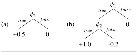
For example, Figure 3 shows a case where NP

classification better served by the informative

con-junctionφ₁∧φ₂found by the decision trees. Given

Figure 3 An example of a decision (a) stump and (b) tree for scoringNP-inferences. Each leaf’s value is the confidence assigned to all inferences that fall in this leaf.φ1 asks “does the first child have a de-terminer headtag?”.φ2asks “does the last child have

a noun label?”.NPclassification is better served by

the informative conjunctionφ1∧φ2found by the de-cision trees.

(a)

φ1 true f alse

+0.5 0

(b)

φ1 true f alse

φ2

true f alse 0

+1.0 -0.2

Table 7 PARSEVAL results of deterministic parsers

on the ≤ 15 words development set through 8700

splits. A shaded cell means that the difference

be-tween this value and that of the baseline is statisti-cally significant. All differences between l2r and r2l are significant.

Dev Dev Dev MRL #splits

LFMS LRCL LPRC Θˆ total

l2r 83.61 82.71 84.54 3.37 2157

r2l 85.76 85.37 86.15 3.39 1881

Baseline 87.07 86.05 88.12 1.92 7283

the sentence “The man left”, at the initial state there

are six candidate NP-inferences, one for each span,

and “(NPThe man)” is the only candidate inference

that is correct.φ1is true for the correct inference and two of the incorrect inferences (“(NPThe)” and “(NP The man left)”).φ1∧φ2, on the other hand, is true only for the correct inference, and so it is better at

discriminatingNPs over this sample.

3.5 Deterministic Parsing

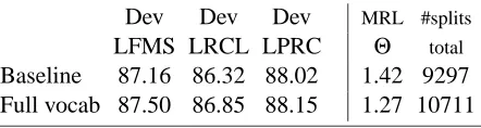
Table 8 PARSEVAL results of the full vocabulary

parser on the≤ 15 words development set. The

dif-ferences between the full vocabulary run and the baseline are not statistically significant.

Dev Dev Dev MRL #splits

LFMS LRCL LPRC Θ total

Baseline 87.16 86.32 88.02 1.42 9297

Full vocab 87.50 86.85 88.15 1.27 10711

parser with at most 8700 splits.

r2l parsing is significantly more accurate than l2r. The reason is that the deterministic runs (l2r and r2l) must avoid prematurely inferring items that come later in the item ordering. This puts the l2r parser in a tough spot. If it makes far-right decisions, it’s more likely to prevent correct subsequent decisions that are earlier in the l2r ordering, i.e. to the left. But if it makes far-left decisions, then it goes against the right-branching tendency of English sentences. In contrast, the r2l parser is more likely to be correct when it infers far-right constituents.

We also observed that the accuracy of the de-terministic parsers dropped sharply as training pro-gressed (See Figure 4). This behavior was

unex-pected, as the accuracy curve levelled offin every

other experiment. In fact, the accuracy of the deter-ministic parsers fell even when parsing the training data. To explain this behavior, we examined the mar-gin distributions of the r2l NP-classifier (Figure 5). As training progressed, theNP-classifier was able to reduce loss by driving up the margins of the incor-rect training examples, at the expense of incorincor-rectly classifying a slightly increased number of correct training examples. However, this is detrimental to parsing accuracy. The more correct inferences with negative confidence, the less likely it is at some state that the highest confidence inference is correct. This effect is particularly pronounced in the deterministic setting, where there is only one correct inference per state.

3.6 Full Vocabulary

As in traditional parsers, the baseline was smoothed by replacing any word that occurs fewer than five

times in the training data with the special tokenUNK

(Table 3.9). Table 8 compares the baseline to a full vocabulary run, in which the vocabulary contained

all words observed in the training data. As evidenced by the results therein, controlling for lexical sparsity did not significantly improve accuracy in our setting. In fact, the full vocabulary run is slightly more ac-curate than the baseline on the development set, al-though this difference was not statistically signifi-cant. This was a late-breaking result, and we used the full vocabulary condition as our final parser for parsing the test set.

3.7 Test Set Results

Table 9 shows the results of our best parser on the

≤15 words test set, as well as the accuracy reported

for a recent discriminative parser (Taskar et al., 2004) and scores we obtained by training and test-ing the parsers of Charniak (2000) and Bikel (2004) on the same data. Bikel (2004) is a “clean room” reimplementation of the Collins parser (Collins, 1999) with comparable accuracy. Both Charniak (2000) and Bikel (2004) were trained using the gold-standard tags, as this produced higher accuracy on the development set than using Ratnaparkhi (1996)’s tags.

3.8 Exploratory Data Analysis

To gain a better understanding of the weaknesses of our parser, we examined a sample of 50 develop-ment sentences that the full vocabulary parser did not get entirely correct. Besides noise and cases of genuine ambiguity, the following list outlines all er-ror types that occurred in more than five sentences, in roughly decreasing order of frequency. (Note that there is some overlap between these groups.)

• ADVPs andADJPs A disproportionate amount of

the parser’s error was due to ADJPs and ADVPs.

Out of the 12.5% total error of the parser on the development set, an absolute 1.0% was due to

ADVPs, and 0.9% due to ADJPs. The parser had

LFMS=78.9%,LPRC=82.5%,LRCL=75.6%

on ADVPs, and LFMS = 68.0%,LPRC =

71.2%,LRCL=65.0% onADJPs.

Figure 4 LFMS of the baseline and the deterministic runs on the≤ 15 words development set of the Penn Treebank. The x-axis shows the LFMS as training progresses and the number of decision tree splits in-creases.

74 76 78 80 82 84 86 88

8700 5000

2500 1000

250

74 76 78 80 82 84 86 88

Parseval FMS

Total # of splits Baseline

Right-to-left Left-to-right

Figure 5 The margin distributions of the r2lNP-classifier, early in training and late in training, (a) over the incorrect training examples and (b) over the correct training examples.

(a)

-20 0 20 40 60 80 100 120 140 160

0 0.1 0.2 0.3 0.4 0.5 0.6 0.7 0.8 0.9 1

Margin

Percentile Late in training Early in training

(b)

-40 -30 -20 -10 0 10 20

0 0.1 0.2 0.3 0.4 0.5 0.6 0.7 0.8 0.9 1

Margin

Percentile Late in training Early in training

The amount of noise present in ADJP andADVP

annotations in the PTB is unusually high.

Annota-tion ofADJPandADVPunary projections is

partic-ularly inconsistent. For example, the development set contains the sentence “The dollar was trading sharply lower in Tokyo .”, with “sharply lower”

bracketed as “(ADVP (ADVP sharply) lower)”.

“sharply lower” appears 16 times in the complete

training section, every time bracketed as “(ADVP

sharply lower)”, and “sharply higher” 10 times,

always as “(ADVPsharply higher)”. Because of the

Table 9 PARSEVAL results of on the≤ 15 words test set of various parsers in the literature. The diff er-ences between the full vocabulary run and Bikel or Charniak are significant. Taskar et al. (2004)’s output

was unavailable for significance testing, but presumably its differences from the full vocab parser are also

significant.

Test Test Test Dev Dev Dev

LFMS LRCL LPRC LFMS LRCL LPRC

Full vocab 87.13 86.47 87.80 87.50 86.85 88.15

Bikel (2004) 88.85 88.31 89.39 86.82 86.43 87.22

Taskar et al. (2004) 89.12 89.10 89.14 89.98 90.22 89.74

Charniak (2000) 90.09 90.01 90.17 89.50 89.69 89.32

bias is to cope with the noise by favoring negative

confidences predictions for ambiguousADJPand

ADVPdecisions, hence their abysmal labelled

re-call. One potential solution is the weight-sharing strategy described in Section 3.5.

• Tagging Errors Many of the parser’s errors

were due to poor tagging. Preprocessing sentence “Would service be voluntary or compulsory ?” gives “would/MD service/VB be/VB voluntary/JJ or/CC UNK/JJ” and, as a result, the parser

brack-ets “service . . . compulsory” as a VP instead of

correctly bracketing “service” as anNP. We also

found that the tagger we used has difficulties with completely capitalized words, and tends to tag

themNNP. By giving the parser access to the same

features used by taggers, especially rich lexical features (Toutanova et al., 2003), the parser might learn to compensate for tagging errors.

• Attachment decisions The parser does not

de-tect affinities between certain word pairs, so it has

difficulties with bilexical dependency decisions.

In principle, bilexical dependencies can be rep-resented as conjunctions of feature given in Sec-tion 2.1.4. Given more training data, the parser might learn these affinities.

4 Conclusions

In this work, we presented a near state-of-the-art approach to constituency parsing which over-comes some of the limitations of other discrimina-tive parsers. Like Yamada and Matsumoto (2003) and Sagae and Lavie (2005), our parser is driven by classifiers. Even though these classifiers themselves never do any parsing during training, they can be combined into an effective parser. We also presented

a beam search method under the objective function of maximizing the minimum confidence.

To ensure efficiency, some discriminative parsers

place stringent requirements on which types of fea-tures are permitted. Our approach requires no such restrictions and our scoring function can, in prin-ciple, use arbitrary information from the history to evaluate constituent inferences. Even though our features may be of too fine granularity to dis-criminate through linear combination, discrimina-tively trained decisions trees determine useful ture combinations automatically, so adding new

fea-tures requires minimal human effort.

Training discriminative parsers is notoriously slow, especially if it requires generating examples by repeatedly parsing the treebank (Collins & Roark, 2004; Taskar et al., 2004). Although training time is still a concern in our setup, the situation is ame-liorated by generating training examples in advance and inducing one-vs-all classifiers in parallel, a tech-nique similar in spirit to the POS-tag parallelization in Yamada and Matsumoto (2003) and Sagae and Lavie (2005).

This parser serves as a proof-of-concept, in that we have not fully exploited the possibilities of en-gineering intricate features or trying more complex

search methods. Its flexibility offers many

oppor-tunities for improvement, which we leave to future work.

Acknowledgments

and constructive criticism. This research was spon-sored by an NSF CAREER award, and by an equip-ment gift from Sun Microsystems.

References

Bikel, D. M. (2004). Intricacies of Collins’ pars-ing model. Computational Lpars-inguistics, 30(4), 479–511.

Black, E., Abney, S., Flickenger, D., Gdaniec, C.,

Grishman, R., Harrison, P., et al. (1991).

A procedure for quantitatively comparing the syntactic coverage of English grammars. In Speech and Natural Language (pp. 306–311). Charniak, E. (2000). A maximum-entropy-inspired

parser. In NAACL (pp. 132–139).

Cohen, P. R. (1995). Empirical methods for artificial intelligence. MIT Press.

Collins, M. (1999). Head-driven statistical models for natural language parsing. Unpublished doctoral dissertation, UPenn.

Collins, M. (2003). Head-driven statistical models for natural language parsing. Computational Linguistics, 29(4), 589–637.

Collins, M., & Koo, T. (2005). Discriminative

reranking for natural language parsing. Com-putational Linguistics, 31(1), 25–69.

Collins, M., & Roark, B. (2004). Incremental pars-ing with the perceptron algorithm. In ACL. Collins, M., Schapire, R. E., & Singer, Y. (2002).

Logistic regression, AdaBoost and Bregman distances. Machine Learning, 48(1-3), 253– 285.

Henderson, J. (2003). Inducing history representa-tions for broad coverage statistical parsing. In HLT/NAACL.

Kalt, T. (2004). Induction of greedy controllers for deterministic treebank parsers. In EMNLP (pp. 17–24).

Kearns, M. J., & Mansour, Y. (1999). On the boost-ing ability of top-down decision tree learnboost-ing algorithms. Journal of Computer and Systems Sciences, 58(1), 109–128.

Klein, D., & Manning, C. D. (2001). Parsing and hypergraphs. In IWPT (pp. 123–134).

Klein, D., & Manning, C. D. (2003). Accurate un-lexicalized parsing. In ACL (pp. 423–430).

Magerman, D. M. (1995). Statistical decision-tree models for parsing. In ACL (pp. 276–283). Marcus, M. P. (1980). Theory of syntactic

recogni-tion for natural languages. MIT Press. Och, F. J., & Ney, H. (2002). Discriminative training

and maximum entropy models for statistical machine translation. In ACL.

Ratnaparkhi, A. (1996). A maximum entropy part-of-speech tagger. In EMNLP (pp. 133–142). Sagae, K., & Lavie, A. (2005). A classifier-based

parser with linear run-time complexity. In

IWPT.

Schapire, R. E., & Singer, Y. (1999). Improved boosting using confidence-rated predictions. Machine Learning, 37(3), 297–336.

Taskar, B., Klein, D., Collins, M., Koller, D., & Manning, C. (2004). Max-margin parsing. In EMNLP (pp. 1–8).

Taylor, A., Marcus, M., & Santorini, B. (2003). The Penn Treebank: an overview. In A. Abeill´e (Ed.), Treebanks: Building and using parsed corpora (pp. 5–22).

Toutanova, K., Klein, D., Manning, C. D., & Singer, Y. (2003). Feature-rich part-of-speech tag-ging with a cyclic dependency network. In HLT/NAACL (pp. 252–259).

Wong, A., & Wu, D. (1999). Learning a

lightweight robust deterministic parser. In

EUROSPEECH.

Yamada, H., & Matsumoto, Y. (2003). Statistical dependency analysis with support vector ma-chines. In IWPT.