Document Clustering with Grouping and Chaining Algorithms

(1)

Chaining Algorithms

Yllias Chali and Souﬁane Noureddine Department of Computer Science,

University of Lethbridge

Abstract. Document clustering has many uses in natural language tools and applications. For instance, summarizing sets of documents that all describe the same event requires ﬁrst identifying and grouping those documents talking about the same event. Document clustering involves dividing a set of documents into non-overlapping clusters. In this paper, we present two document clustering algorithms:grouping algorithm, and

chaining algorithm. We compared them with k-means and the EM algo-rithms. The evaluation results showed that our two algorithms perform better than the k-means and EM algorithms in diﬀerent experiments.

1 Introduction

Document clustering has many uses in natural language tools and applications. For instance, summarizing sets of documents that all describe the same event requires ﬁrst identifying and grouping those documents talking about the same event. Document clustering involves dividing a set of texts into non-overlapping clusters, where documents in a cluster are more similar to one another than to documents in other clusters. The term moresimilar, when applied to clustered documents, usually means closer by some measure of proximity or similarity.

According to Manning and Schutze [1], there are two types of structures pro-duced by clustering algorithms, hierarchical clustering and ﬂat or non-hierarchical clustering. Flat clustering are simply groupings of similar objects. Hierarchical clustering is a tree of subclasses which represent the cluster that contains all the objects of its descendants. The leaves of the tree are the individ-ual objects of the clustered set. In our experiments, we used the non-hierarchical clustering k-means and EM [2] and our own clustering algorithms.

There are several similarity measures to help ﬁnd out groups of related doc-uments in a set of docdoc-uments [3]. We use identical word method and semantic relation method to assign a similarity score to each pair of compared texts. For the identical word method, we use k-means algorithm, the EM algorithm, and our owngrouping algorithmto cluster the documents. For the semantic relation method, we use our owngrouping algorithmandchaining algorithm to do the clustering job. We choose WordNet 1.6 as our background knowledge. WordNet consists of synsets gathered in a hypernym/hyponym hierarchy [4]. We use it to get word senses and to evaluate the semantic relations between word senses. R. Dale et al. (Eds.): IJCNLP 2005, LNAI 3651, pp. 280–291, 2005.

c

(2)

2 Identical Word Similarity

To prepare the texts for the clustering process using identical word similarity, we perform the following steps on each of the selected raw texts:

1. Preprocessing which consists in extracting ﬁle contents from the raw texts, stripping special characters and numbers, converting all words to lower cases and removing stopwords, and converting all plural forms to singular forms. 2. Create document word vectors: each document was processed to record the

unique words and their frequencies. We built the local word vector for each document, each vector entry will record a single word and its frequency. We also keep track of the unique words in the whole texts to be tested. After processing all the documents, we convert each local vector to a global vector using the overall unique words.

3. Compute the identical word similarity score among documents: given any two documents, if we have their global vectors x,y, we can use the cosine measure [5] to calculate the identical word similarity score between these two texts.

cos(x,y) =

n i=1xiyi

n

i=1x 2

i

n

i=1y 2

i

(1)

wherexandyare n-dimensional vectors in a real-valued space.

Now, we determined a global vector for each text. We also have the identical word similarity scores among all texts. We can directly use these global vectors to run the k-means or the EM algorithms to cluster the texts. We can also use the identical word similarity scores to rungrouping algorithm(deﬁned later) to do the clustering via a diﬀerent approach.

3 Semantic Relation Similarity

To prepare the texts for clustering process using semantic relation similarity, the following steps are performed on each raw texts:

1. Preprocessing which consists in extracting ﬁle contents, and removing special characters and numbers.

(3)

Wordnet. When we get a noun (or a compound noun) existing in WordNet, we insert it into the meaningful word set, which we call set of regular nouns, otherwise we insert it into the non-meaningful word set, which we call set of proper nouns.

During the processing of each document, we save the over-all unique meaningful nouns in an all regular nouns set. Because of the big over-head related to accessing WordNet, we try to reduce the overall access times to a minimal level. Our approach is to use these over-all unique nouns to retrieve the relevant information from WordNet and save them in a global ﬁle. For each sense of each unique noun, we save its synonyms, two level hypernyms, and one level hyponyms. If any process frequently needs the WordNet information, it can use the global ﬁle to store the information in a hash and thus provides fast access to its members.

3. Word sense disambiguation.

Similarly to Galley and McKeown [6], we use lexical chain approach to disambiguate the nouns in the regular nouns for each document [7,8]. A lexical chain is a sequence of related words in the text, spanning short (adjacent words or sentences) or long distances (entire text). WordNet is one lexical resource that may be used for the identiﬁcation of lexical chains. Lexical chains can be constructed in a source text by grouping (chaining) sets of word-senses that are semantically related. We designate the following nine semantic relations between two senses:

(a) Two noun instances are identical, and used in the same sense; (b) Two noun instances are used in the same sense (i.e., are synonyms );

(c) The senses of two noun instances have a hypernym/hyponym relation between them;

(d) The senses of two noun instances are siblings in the hypernym/hyponym tree;

(e) The senses of two noun instances have a grandparent/grandchild relation in the hypernym/hyponym tree;

(f) The senses of two noun instances have a uncle/nephew relation in the hypernym/hyponym tree;

(g) The senses of two noun instances are cousins in the hypernym/hyponym tree (i.e., two senses share the same grandparent in the hypernym tree of WordNet);

(h) The senses of two noun instances have a great-grandparent/great-child relation in the hypernym/hyponym tree (i.e., one sense’s grand-parent is another sense’s hyponym’s great-grandgrand-parent in the hypernym tree of WordNet).

(i) The senses of two noun instances do not have any semantic relation. To disambiguate all the nouns in the regular nouns of a text, we proceed with the following major steps:

(4)

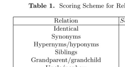
the following scoring scheme for the relations deﬁned above as shown in Table 1. The score betweenAi(senseiof wordA) andBj(sensejof word

B) is denoted asscore(Ai, Bj). These scores are established empirically

[image:4.512.111.320.136.248.2]

and give more weight to closer words according to WordNet hierarchy.

Table 1. Scoring Scheme for Relations

Relation Score(Ai, Bj)

Identical log(16)

Synonyms log(15)

Hypernyms/hyponyms log(14)

Siblings log(13)

Grandparent/grandchild log(12) Uncle/nephew log(11)

Cousins log(10)

Great-grandparent/great-grandchild log(9)

No relation 0

(b) Build the lexical chains using all possible senses of all nouns. To build the lexical chains, we assume each noun possesses all the possible senses from WordNet. For each sense of each noun in a text, if it is related to all the senses of any existing chain, then we put this sense into this chain, else we create a new chain and push this sense into the new empty chain. After this, we will have several lexical chains with their own scores. (c) Using the lexical chain, try to assign a speciﬁc sense to each nouns.

We sort the chains by their scores in a non-increasing order. We select the chain with the highest score and assign the senses in that chain to the corresponding words. These words are disambiguated now. Next, we process the next chain with the next highest score. If it contains a diﬀerent sense of any disambiguated words, we skip it to process the next chain until we reach the chains with a single entry. We mark the chains which we used to assign senses to words as selected. For the single entry chains, if the sense is the only sense of the word, we mark it as disambiguated. For each undisambiguated word, we check each of its senses against all the selected chains. If it has a relation with all the senses in a selected chain, we will then remember which sense-chain pair has the highest relation score, then we assign that sense to the corresponding word.

After these steps, the leftover nouns will be the undisambiguated words. We save the disambiguated words and the undisambiguated words with their frequencies for calculating the semantic relation scores between texts. 4. Compute the similarity score for each pair of texts.

(5)

between each pair of texts. For the purpose of calculating the semantic sim-ilarity scores among texts, we use only the ﬁrst three relations (a), (b), and (c) and the last relation (i) and their corresponding scores deﬁned inTable 1. For a given text pair, we proceed as in the following steps to calculate the similarity scores:

– Using the disambiguated nouns, the score score1 of the similarity be-tween two textsT1 andT2is computed as follows:

score1= n

i=1

m

j=1score(Ai, Bj)×f req(Ai)×f req(Bj)

n

i=1f req2(Ai)

m

j=1f req2(Bj)

(2)

where Ai is a word sense from T1 and Bj is a word sense from T2;

score(Ai, Bj) is a semantic relation score deﬁned in Table 1; n and m

are the numbers of disambiguated nouns in T1 and T2; f req(x) is the frequency of a word sensex.

– For the undisambiguated nouns, if two nouns are identical in their word formats, then the probability that they take the same sense in both texts is 1/s, where s is the number of their total possible senses. The similarity score score2 between two texts T1 and T2 according to the undisambiguated nouns is computed as follows:

score2= n

i=1

log(16)×f req1(Ai)×f req2(Ai) si

n

i=1f req 2 1(Ai)

n

j=1f req 2 2(Aj)

(3)

whereAi is a word common toT1 and T2; nis the number of common

words toT1andT2;f req1(Ai) is the frequency ofAiinT1;f req2(Ai) is

the frequency ofAi in T2;si is the number of senses ofAi.

– The proper nouns are playing an important role in relating texts to each other. So, we use a higher score (i.e.,log(30)) for the identical proper nouns. The similarity scorescore3 between two texts T1and T2 among the proper nouns between is computed as follows:

score3= n

i=1log(30)×f req1(Ai)×f req2(Ai)

n

i=1f req21(Ai)

n

j=1f req22(Aj)

(4)

where Ai is a proper noun common to T1 and T2; n is the number of common proper nouns toT1andT2;f req1(Ai) is the frequency ofAiin

T1;f req2(Ai) is the frequency ofAi in T2.

– Adding all the scores together as the total similarity score of the text pair:

score=score1+score2+score3 (5) Now we make it ready to use thegrouping algorithm orchaining algorithm

(6)

4 Clustering Algorithms

Generally, every text should have a higher semantic similarity score with the texts from its group than the texts from a diﬀerent groups [9]. There are a few rare cases where this assumption could fail. One case is that the semantic similarity score does not reﬂect the relationships among the texts. Another case is that the groups are not well grouped by common used criteria or the topic is too broad in that group.By all means, the texts of any well formed clusters should have stronger relations among its members than the texts in other clusters. Based on this idea, we developed two text clustering algorithms:grouping algorithm

and chaining algorithm. They share some common features but with diﬀerent approaches.

One major issue in partitioning texts into different clusters is choosing the cutoff on the relation scores. Virtually, all texts are related with each other to some extent. The problem here is how similar (or close) they should be so that we can put them into one cluster and how dissimilar (or far away) they should be so that we can group them into different clusters. Unless the similarity scores among all the texts can be represented as binary values, we will always face this problem with any kind of texts. In order to address this problem, we introduce two reference values in our text clustering algorithms:high-threshold and low-threshold. The high-threshold means the high standard for bringing two texts into the same cluster. The low-threshold means the minimal standard for possibly bringing two texts into the same cluster. If the score between any two texts reaches or surpasses the high-threshold, then they will go to the same cluster. If the score reaches the low-threshold but is lower than the high-threshold, then we will carry out further checking to decide if we should bring two texts into the same cluster or not, else, the two texts will not go to the same cluster.

We get our high-threshold and low-threshold for our diﬀerent algorithms by running some experiments using the grouped text data. The high-threshold we used for our two algorithms is 1.0 and the low-threshold we used is 0.6. For our experiment, we always take a number of grouped texts and mix them up to make a testing text set. So, each text must belong to one cluster with certain number of texts.

4.1 Grouping Algorithm

The basic idea is that each text could gather its most related texts to form an initial group, then we decide which groups have more strength over other groups, make the stronger groups as ﬁnal clusters, and use them to bring any possible texts to their clusters. First, we use each text as a leading text (Tl) to

form a cluster. To do this, we put all the texts which have a score greater than the high-threshold with Tl into one group and add each score to the group’s

(7)

with the highest score and check if any text in this group has been clustered to the existing final clusters or not. If not more than 2 texts are overlapping with the final clusters, then we take this group as a final cluster, and remove the overlapping texts from other final clusters. We process the group with the next highest score in the same way until the groups’ entries are less than 4. For those groups, we would first try to insert their texts into the existing final clusters if they can fit in one of them. Otherwise, we will let them go to the leftover cluster which holds all the texts that do not belong to any final clusters. The following is the pseudocode for the grouping algorithm:

Grouping Algorithm

// Get the initial clusters for each textti

construct a text cluster including all the texts(tj)

which score(ti, tj)>= high-threshold;

compute the total score of the text cluster;

ﬁnd out its neighbor with maximum relation score; end for

// Build the ﬁnal clusters

sort the clusters by their total score in non-increasing order; for each clustergi in the sorted clusters

if member(gi)>3 and overlap-mem(gi)<= 2

takegi as a ﬁnal clusterci;

mark all the texts inci as clustered;

else

skip to process next cluster; end if

end for

// Process the leftover texts and insert them into one of the ﬁnal clusters for each texttj

iftj has not been clustered

ﬁnd cluster ci with the highest score(ci,tj);

if the average-score(ci,tj)>= low-threshold

puttj into the clusterci;

else if the max score neighbortm oftj is inck

puttj into clusterck;

else

puttj into the ﬁnal leftover cluster;

end if end if end for

(8)

where: member(gi) is the number of members in groupgi; overlap-mem(gi) is

the number of members that are overlapped with any ﬁnal clusters; score(ci,

tj) is the sum of scores between tj and each text in ci; average-score(ci, tj) is

score(ci,tj) divide by the number of texts inci.

4.2 Chaining Algorithm

This algorithm is based on the observation of the similarities among the texts in groups. Within a text group, not all texts are always strongly related with any other texts. Sometimes there are several subgroups existing in a single group, i.e., cer-tain texts have stronger relations with their subgroup members and have a weaker relation with other subgroup members. Usually one or more texts have stronger relation crossing diﬀerent subgroups to connect them together, otherwise all the texts in the group could not be grouped together. So, there is a chaining eﬀect in each group connecting subgroups together to form one entire group.

We use this chaining idea in thechaining algorithm. First, for each textTj,

we ﬁnd all the texts which have similarity scores that are greater or equal than the high-threshold withTj and use them to form a closer-text-set. All the texts

in that set are called closer-text ofTj.

Next, for each text which has not been assigned to a final chain, we use its initial closer-text-set members to form a new chain. For each of the texts in the chain, if any of its closer-texts are relatively related (i.e., the score>= low-threshold) to all the texts in the chain, then we add it into the current chain. One thing needs to be noticed here is that we do not want to simply bring all the closer-texts of each current chain’s members into the chain. The reason is to eliminate the unwanted over-chaining effect that could bring many other texts which are only related to one text in the existing chain. So, we check each candidate text against all the texts in the chain to prevent the over-chaining effect. We repeat this until the chain’s size are not increasing. If the chain has less than 4 members, we will not use this chain for a final cluster and try to re-assign the chain members to other chains.

After the above process, if any text has not been assigned to a chain we check it against all existing chains and ﬁnd the chain which has highest similarity score between the chain and this text. If the average similarity score with each chain members is over low-threshold, we insert this text into that chain, else we put it into the ﬁnal leftover chain. The following is the pseudocode for the chaining algorithm:

5 Application

(9)

Chaining Algorithm

// construct a closer-text-set for each text for each textti0< i <=N

for each texttj 0< j <=N if score(ti,tj)>= high-threshold

puttj into closer-text-setsi; end if

end for end for

// Build the chains c = 0;

for each texttiof all the texts if it has not been chained in

put texttiinto chain c and mark it as been chained; bring all the text in closer text-setsiinto the new chain c; marksias processed;

while (the size of chain c is changing) for each texttk in chain c

for each texttminsk oftk

if the score betweentmand any text in chain c>= low-threshold puttminto chain c;

marktm as been chained to chain c; end if

end for end for end while

if the size of chain c<4 discard chain c;

remark the texts in chain c as unchained; end if

c++; end if end for

// Process the leftover texts and insert them into one of the existing chains for each unchained texttj

ﬁnd chainci with the highest score(ci,tj); if the average-score(ci,tj)>= low-threshold

puttjinto the chainci; else

puttjinto the ﬁnal leftover chain; end if

end for

(10)

algorithm. Then, we measure how successful are these algorithms in reconstitut-ing the original directories. We implemented thek-means algorithmand theEM algorithm to compare them with our algorithms.

In our test, we found out that the chaining algorithm did not work well for identical method. We tested grouping algorithm, chaining algorithm, and EM algorithm with semantic method, and k-means algorithm, EM algorithm, and grouping algorithm with identical methods. We run the k-means and the EM algorithms 4 times with each experiment texts set and take the average performance. As we described before, semantic method represents text relations with scores, so k-means algorithm which needs input data in vector format will not be applied to semantic method.

6 Evaluation

For our testing, we need to compare the system clusters with the testing clusters (original text directories) to evaluate the performance of each system. We ﬁrst compare each system cluster with all of the testing clusters to ﬁnd the best matched cluster pair with the maximum number of identical texts. We then use recall, precision, and F-value to evaluate each matching pair. Finally, we use the average F-value to evaluate the whole system performance. For a best matched pairT Cj(testing cluster) andSCi(system cluster), the recall (R), precision (P),

and F-value (F) are deﬁned as follows:

R=m

t (6)

P = m

m+n (7)

F(T Cj, SCi) =

2P R

P+R (8)

wheremis the number of the overlapping texts betweenT Cj andSCi;nis the

number of the non-overlapping texts in SCi; t is the total number of texts in

T Cj.

For the whole system evaluation, we use theAverage F which is calculated using the F-values of each matched pair of clusters.

Average F =

i,jmax(F(SCi, T Cj))

max(m, n) (9)

(11)

7 Results

The performance of grouping algorithm and chaining algorithm are very close using the semantic relation approach and most of their Average F are over 90%. For the identical word approach, the grouping algorithm performance is much better than the performances of the k-means algorithm and the EM algorithm. The poor performance of the k-means algorithm results from ran-domly selected k initial values. Those initial N-dimensional values usually do not represent the whole data very well. For the semantic relation approach, both grouping and chaining algorithms performed better than the EM algorithm.

[image:11.512.159.268.273.307.2]

Table 2 and 3 are the systemAverage F values for the diﬀerent algorithms. The identical word similarity method used grouping algorithm, k-means rithm, and EM algorithm. The semantic similarity method used grouping algo-rithm, chaining algorithm and EM algorithm.

Table 2.Comparisons of F-value using Identical Word Similarity

Identical Word Similarity Grouping EM k-means

0.98 0.81 0.66

Table 3.Comparisons of F-value using Semantic Relation Similarity

Semantic Relation Similarity Grouping Chaining EM

0.92 0.91 0.76

8 Conclusion

Document clustering is an important tool for natural language applications. We presented two novel algorithms grouping algorithm and chaining algorithm for clustering sets of documents, and which can handle a large set of documents and clusters. The two algorithms use semantic similarity and identical word measure, and their performance is much better than the performance of the K-means algorithm and the performance of the EM algorithm, used as a baseline for our evaluation.

Evaluating the system quality has been always a diﬃcult issue. We presented an evaluation methodology to assess how the system clusters are related to the manually generated clusters using precision and recall measures.

(12)

Acknowledgments

This work was supported by the Natural Sciences and Engineering Research Council (NSERC) research grant.

References

1. Manning, C.D., Schutze, H.: Foundations of Statistical Natural Language Process-ing. MIT Press (2000)

2. Berkhin, P.: Survey of clustering data mining techniques. Technical report, Accrue Software, San Jose, CA (2002)

3. Duda, R., Hart, P.: Pattern Classiﬁcation and Scene Analysis. John Wiley & Sons, New York, NY (1973)

4. Miller, G.A., Beckwith, R., Fellbaum, C., Gross, D., Miller, K.: Five papers on wordnet. CSL Report 43, Cognitive Science Laboratory, Princeton University (1993)

5. Salton, G.: Automatic Text Processing: The Transformation, Analysis, and Re-trieval of Information by Computer. Addison-Wesley Series in Computer Sciences (1989)

6. Galley, M., McKeown, K.: Improving word sense disambiguation in lexical chaining. In: Proceedings of the 18th International Joint Conference on Artiﬁcial Intelligence, Acapulco, Mexico. (2003)

7. Barzilay, R., Elhadad, M.: Using lexical chains for text summarization. In: Pro-ceedings of the 35th Annual Meeting of the Association for Computational Linguis-tics and the 8th European Chapter Meeting of the Association for Computational Linguistics, Workshop on Intelligent Scalable Text Summarization, Madrid (1997) 10-17

8. Silber, H.G., McCoy, K.F.: Eﬃciently computed lexical chains as an intermediate representation for automatic text summarization. Computational Linguistics 28 (2002) 487–496

9. Pantel, P., Lin, D.: Document clustering with committees. In: Proceedings of the ACM SIGIR’02, Finland (2002)

10. Over, P., ed.: Proceedings of the Document Understanding Conference, NIST (2003)