H
-Matrix Arithmetic for Fast Direct and Iterative Method
of Moment Solution of Surface-Volume-Surface EFIE
for 3-D Radiation Problems
Reza Gholami1, *, Jamiu Mojolagbe1, Anton Menshov2, Farhad S. H. Lori1, and Vladimir Okhmatovski1
Abstract—Hierarchical (H-) matrix based fast direct and iterative algorithms are presented for acceleration of the Method of Moment (MoM) solution of the Surface-Volume-Surface Electric Field Integral Equation (SVS-EFIE) formulated for scattering and radiation problems on homogeneous dielectric objects. As the SVS-EFIE features the product of the integral operator mapping the tangential equivalent electric current on the surface of the scatterer to the volume polarization current and the integral operator mapping the volume polarization current to the tangential component of the scattered electric field, its MoM discretization produces the product of non-square matrices. Formation of the non-square H-matrices for the MoM discretized integral operators is described. The algorithms for arithmetics pertinent to the product of the non-square H-matrices are explained. The memory and CPU time complexity scaling of the required H-matrix operations are analyzed in details and verified numerically. The numerical validation of the proposed algorithm is provided for both the low-loss dielectric objects as well as for the high-low-loss biological tissues found in the bioelectromagnetics applications. The numerical experiments demonstrate a significant reduction of memory usage and a considerable speedup for CPU time compared to na¨ıve MoM, thus, enabling solution of the large-scale scattering and radiation problems with the SVS-EFIE.
1. INTRODUCTION
Electromagnetic field interactions with the biological tissues occur in many natural and staged scenarios ranging from involuntary human body exposures to the natural and man-made sources of RF and microwave radiation [1] to the near field radiation of the mobile [2], wearable and implanted antennas [3] or biomedical imaging systems [4]. Understanding, prediction, and control of such interactions is becoming of paramount importance in the design of the novel body mounted communication systems [5] and sensor networks [6], setting up the Internet-of-Things connected home and office spaces [7], development of smart antennas for 5G systems [8], and many other practical applications [9].
The limiting capabilities of the non-invasive experimental techniques for studies of field-to-body interactions motivate development of computational methods [10] for accurate virtual prototyping of such phenomenon. Due to significant inhomogeneity of the biological tissues, the methods of computational electromagnetics (CEM) based on the direct discretization of the Maxwell Equations such as Finite-Difference Time-Domain (FDTD) [11] and discretization of the wave equations such as the Finite Element Method (FEM) [12] have become the most popular approaches for bioelectromagnetics (BioEM) analysis with various commercial tools available [13, 14]. While FDTD and FEM offer great
Received 19 October 2018, Accepted 28 November 2018, Scheduled 7 December 2018 * Corresponding author: Reza Gholami ([email protected]).
1 Department of Electrical and Computer Engineering, University of Manitoba, Winnipeg, MB R3T 5V6, Canada. 2 Department of
versatility and simplicity in implementation and parallelization, they are plagued by fundamental limitations of error accumulation when propagation of wave phenomena over electrically large distances is analyzed [15] and necessity to discretize the space outside the regions of interest [12]. Integral equations (IEs) of CEM discretized with Method of Moments (MoM) [16] establish computational frameworks free of these disadvantages. The discretization of the IEs, however, results in the dense matrix equations which require development of sophisticated fast algorithms [15] in order to reduce the CPU time and memory complexity associated with their solution. The detailed comparisons in terms of the achieved accuracy and used computational resources between the differential and integral equations based approaches in application to solution of the BioEM problems can be found in [17].
The development of fast algorithms aiding iterative solutions of the dense matrix equations [18, 19] which result from the discretization of the IEs has reached a certain maturity [15] with Multi-Level-Fast-Multipole-Method (MLFMM) [20–23], FFT-based methods [24–26], and Adaptive Cross Approximation (ACA) [27, 28] methods dominating the field. The grand challenge in use of the fast iterative algorithms though is in development of appropriate preconditioning schemes which ensure sufficiently rapid convergence under conditions of multiscale discretization, high disparity in the material properties, and broad range of frequencies. To date development of such preconditioning schemes has been met with only partial success and remains a rather ’black art’ than science [29].
The recent efforts in circumventing this grand challenge posed by the lack of robustness in the iterative schemes for the solution of the dense matrix equations have been in two areas. The first is the construction of well-conditioned IE formulations and their appropriate discretization schemes [30], and the second is the development of the fast methods for direct solution of the dense matrix equations [31– 38]. The non-iterative nature of the latter allows them to remain largely insensitive to the deterioration of the IEs conditioning stemming from the multiscaling and other factors and, hence, provide robust computational schemes under conditions where traditional iterative schemes fail.
In this work, we develop a hierarchical (H-) matrix based MoM frameworks [31, 32] for solution of the Surface-Volume-Surface Electric Field Integral Equation (SVS-EFIE) which we recently introduced for analysis of the scattering problems on dielectric objects [39–43]. The SVS-EFIE is a class of Single-Source Surface Integral Equations (SSSIE) [44, 45] which reduces the number of unknowns by half compared to the traditional surface integral-equation formulations [46, 47]. It features only one product of electric-field type integral operators and allows for a mixed potential formulation free of hyper-singular integrals under MoM discretization. These benefits of the SVS-EFIE come at an extra cost of computing field translations from the scatterer surface to its volume and then from its volume back to the surface. In the BioEM applications, computation of the field throughout the volume of the lossy body tissues is typically required for determining of the specific absorption rate, depth of field penetration, and localization of the high field concentration areas making SVS-EFIE particularly suitable [43] for solution of such problems. Due to field translation to the volume of the object of interest, discretization of both surface and volume field quantities takes place in the SVS-EFIE. As such, the memory requirements and computational complexity of dense matrix operations and storage for na¨ıve MoM solution of the SVS-EFIE become prohibitive for tackling of practically important problems. To reduce the computational and memory costs, an H-matrix based fast direct and iterative solvers are developed in this work to accelerate MoM solution of the SVS-EFIE for 3-D scattering problems on dielectric objects.
2. FORMULATIONS AND EQUATIONS OF SVS-EFIE AND ITS MOM SOLUTION
In our previous work [40, 43], we introduced a new type of an SSSIE by combining the ideas of the traditional volume equivalence principle and the theory of SSIEs. The SVS-EFIE formulation for 3-D scattering problem is given by Eq. (1), whereris an observation location on the scatterer boundary∂V;
r is the position-vector of the total electric field inside the scatterer; and complex relative permittivity
is =ε+σ/(iωε0). In Eq. (1), ˆt is the tangential vector to the scatterer surface ∂V, and ω is the
cyclic frequency.
iωμ0ˆt·
−
∂V
¯ ¯
G(r,r)·J(r)ds+k20(−1)
V
¯ ¯
G0(r,r)·
∂V
¯ ¯
G(r,r)·J(r)dsdv
=ˆt·Einc(r), r∈∂V.
It is convenient to express Eq. (1) in the integral-operator form
−T,∂V,∂V∇Φ +TTT∂V,∂V,A
T∂V,∂V
◦J+
TTT∂V,V0,∇ϕ+TTT∂V,V0,a
T0∂V,V
◦TTTV,∂V,∇Φ +T,AV,∂V
TV,∂V
◦J =ˆt·Einc,
(2)
where T∂V,∂V, T0∂V,V, and TV,∂V are surface-to-surface, volume-to-surface, and surface-to-volume operators, respectively. Operators T∂V,∂V, T0∂V,V, and TV,∂V in Eq. (2) are composed as a sum of two integral operators corresponding to the scalar and vector potentials as detailed in [40].
In order to solve SVS-EFIE in Eq. (1) with MoM, the volume of the scatterer V is discretized with a 3-D mesh consisting of N tetrahedron elements, and its surface ∂V is discretized with a 2-D mesh consisting ofM triangle elements. Discretization of the unknown tangential weighting functionJ defined on the boundary∂V is performed over P Rao-Wilton-Glisson (RWG) basis functions [48] as
J(r)∼=
P
m=1
Imtm(r). (3)
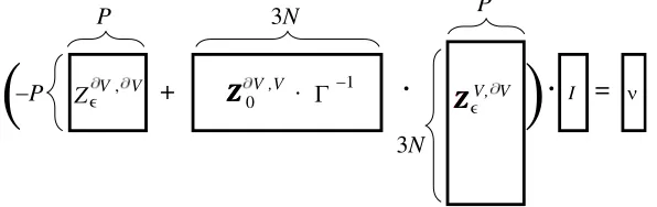
Following the standard MoM procedure (described in detail in [40]), the SVS-EFIE is reduced to the set of linear algebraic equations with respect to the unknown coefficients vector I in the expansion of the unknown surface weighting function in Eq. (3). The MoM matrix equation structure is shown in Fig. 1.
The surface-to-surface impedance matrix Z∂V,∂V corresponding to the operatorT∂V,∂V is a P×P
square matrix since the surface ∂V serves as support for both the domain and range ofT∂V,∂V. The x,
y, andzcomponents ofZZZ∂V,V0 , translating the volume polarization current to the tangential component
of the scattered electric field andZZZV,∂V translating the unknown tangential weighting source function to the total field inside the scatterer are handled separately and result in P ×3N and 3N ×P sized matrices. These matrices have rectangular structures since their continuous counterparts have different range and domain supports: ∂V and V forT0∂V,V and V and ∂V for TV,∂V, respectively. In Fig. 1, Γ is the Gram matrix with elements of Γn,n =Vn, ifn=n and zero, otherwise, n= 1, . . . , N. Here,Vn
is the volume of the nth tetrahedron element.
Z V, V −P
P
+ ZZZ V ,V0 · Γ−1
·
3N3N Z
Z
ZV, V
·
I = νP
∋ ∋
(
(
Figure 1. System of linear equations structure resulting from MoM discretization of the SVS-EFIE (1). Here,P is the number of RWG basis functions on the boundary∂V andN is the number of tetrahedron elements in the volumeV.
3. H-MATRIX ACCELERATION OF MOM SOLUTION
3.1. Multilevel Geometry Partitioning
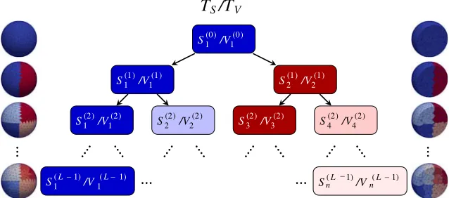
TheH-matrix based MoM algorithm starts with a multilevel partitioning of discretized domains. In this work, we use geometric based bisection [32] that performs well for relatively uniform meshes. Since two different domains ∂V and V are discretized, two separate cluster trees are created: binary tree TS for the test functions and binary treeTV for the basis functions (Fig. 2). To construct a surface cluster tree
TS, we start from the full index set of RWG basis/testing functionsS1(0) (the superscript represents the
level and the subscript represents the ID of the set within the level). Next, we determine the bounding box for this set and partition it in half along the largest dimension to form disjoint children clustersS1(1)
and S2(1). The partitioning process is repeated recursively until the number of basis/testing functions
becomes less than the predetermined leafsize nmin parameter which controls the depth of the cluster
tree. The leafsizenmin is usually chosen empirically, and it is problem/hardware dependent. The cluster
tree for the volume domainTV is constructed similarly toTS with the piece-wise basis/testing functions on the tetrahedron elements being partitioned as opposed to the RWGs. As depicted in Fig. 2, both surface and volume basis/testing functions are hierarchically divided into anL-level tree of clusters. In the subsequent discussion, the levelrelative of the clusterS(j)at thejth level is denoted asR(S(j)).†
S(0)1 /V1(0)
S1(1)/V1(1) S2(1)/V2(1)
S(2)1 /V1(2) S2(2)/V2(2) S3(2)/V3(2) S(2)4 /V4(2)
S1(L−1)/V1(L− 1) Sn(L 1)/V
(L−1)
n
T
S/T
V−
Figure 2. Hierarchical partitioning of RWG basis/testing functions for surface mesh and piece-wise basis/testing functions for volume mesh into an L-level hierarchy of clusters. TS and TV represent surface and volume cluster trees, respectively.
3.2. H-Matrix Structure for the SVS-EFIE Operators
To approximate the impedance matrices of the MoM discretized SVS-EFIE integral operators, the hierarchical matrix structure for each impedance matrix is constructed. The process starts by taking the root elements of the cluster trees corresponding to the range (observer) and domain (source) of the MoM discretized integral operator. The distance between the source and observer, and the size of the individual clusters are calculated, and their interaction is classified as admissible or inadmissible according to the following criterion [31]
min{diam(Bobs),diam(Bsrc)} ≤η dist(Bobs,Bsrc) (4)
where Bobs and Bsrc are the bounding boxes of the observer and source clusters, respectively; diam(·)
and dist(·,·) denote the Euclidean diameter and minimum distance between these bounding boxes. In Eq. (4), parameter η is a positive real number that controls the amount of admissible blocks and accuracy of the solver. The interactions between the test/basis functions in the clusters are considered admissible (corresponding matrix block is rank-deficient), if the distance between the bounding boxes
† Terminology: Relatives of a cluster at all levelshigher than its own levelj (i.e., < j) are calledancestors. For example, for
clusterS1(2)in Fig. 2, its relativeR0(S1(2)) at level 0 isS1(0), e.g.,R0(S1(2)) =S(0)1 . Similarly, level 1 relativeR1(S1(2)) ofS(2)1 isS1(1). Relatives of a cluster at its own level (i.e.,=j)R2(S(2)1 ) ={S1(2), S2(2)}are the cluster itself and itssiblingR2(S1(2)) =S2(2). Also,
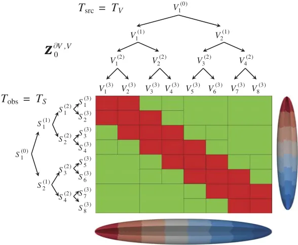
is sufficiently large in Eq. (4). Otherwise, the interactions at this level are classified as inadmissible and interactions between all the children of both the source and observer clusters are examined on admissibility recursively until the leaf level is reached. To demonstrate the described process, the construction ofH-matrix structure for the volume-to-surface operatorZZZ∂V,V0 of SVS-EFIE is visualized
in Fig. 3. Here, the spheroid model [17] is chosen as an example, and four-level surface and volume cluster trees for its test and basis functions are constructed. As demonstrated in Fig. 3, to construct an H-matrix structure forZZZ∂V,V0 ,TS is chosen as the observer tree Tobs and TV chosen as the source tree
Tsrc. The process starts from the interaction between the whole set of surface testing functionsS (0) 1 and
volume basis functionsV1(0) and continues recursively by applying admissibility criterion in Eq. (4).
S1(0)
S(1)2
S(1)1
S4(2)
S3(2)
S2(2)
S1(2)
S(3)8
S(3)7
S(3)6
S(3)5
S(3)4
S(3)3
S(3)2
S(3)1
V1(0)
V2(1) V1(1)
V4(2) V3(2)
V2(2) V1(2)
V8(3)
V7(3)
V6(3)
V5(3)
V4(3)
V3(3)
V2(3)
V1(3) Tsrc = TV
Tobs = TS
ZZZ V ,V0
Figure 3. H-matrix representation of the volume-to-surface MoM impedance matrix ZZZ∂V,V0 arising
from TS×V interaction tree. The structure is constructed using an spheroid model with its surface tree
TS as observer tree and volume tree TV as source tree with tree depth L = 3. Red blocks represent
inadmissible blocks and green blocks represent admissible blocks.
To solve the SVS-EFIE,H-matrix structures have to be constructed for each of the three operators (Fig. 1):
• Z∂V,∂V: TS is chosen for both source Tsrc and observerTobs trees. Therefore, as shown in Fig. 4,
the corresponding surface-to-surface square H-matrix arising from TS×S interaction tree has the
total size of P×P.
• ZZZ∂V,V0 : For volume-to-surface interactions,Tsrc=TV andTobs =TS. The corresponding rectangular
H-matrix arising fromTS×V interaction tree is shown in Fig. 4 and has the total size ofP ×3N. • ZZZV,∂V : For surface-to-volume interactions,Tsrc=TS andTobs =TV. Therefore, as shown in Fig. 4,
the volume-to-surface rectangular H-matrix arising from TV×S interaction tree has the total size of 3N ×P.
3.3. Filling H-Matrices of the SVS-EFIE Operators
ZSV S
P ×P
=
P× P
Z V , V
Zx V ,V0
Z Z Z V ,V0
Zy V ,V0 Zz V ,V0
P× 3N Z
xV,
ZyV,
Z ZZV,
ZzV,
3N ×P
⊗ ⊗
∋
∋
∋ V
V
V
V ∋
∋
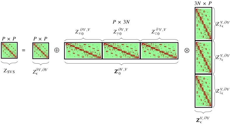
Figure 4. Assembly ofZSVS MoMH-matrix from the individualH-matrices of SVS-EFIE operators:
Z∂V,∂V arising fromTS×S interaction tree,ZZZ∂V,V0 arising fromTS×V, and ZZZV,∂V arising fromTV×S via
formatted multiplication and addition (8) required by aH-LU based direct solution of the SVS-EFIE.
to admissible interactions, ACA algorithm [27] is used to obtain the blocks in a compressed low-rank (R) format:
R
m×n,k(τACA)
= A
m×k(τACA)
× BH
n×k(τACA)
(5)
where m and nare the row and column sizes of the block, and k(τACA) is the revealed rank with the
accuracy of the approximation controlled by the ACA truncation threshold τACA. The complexity of
the ACA is linearly proportional to the size of the block and reveals rankk(τACA) [27].
4. H-MATRIX FAST ITERATIVE AND DIRECT SOLUTIONS
After H-matrix approximations are constructed for each discretized integral operator entering SVS-EFIE, the resultant system of linear algebraic equations
Z∂V,∂V ⊕ZZZ∂V,V0 ⊗ZZZV,∂V
⊗I =V, (6)
has to be solved, with⊗and⊕being the operations of formatted multiplication and addition described later in this section. In this paper, we consider both H-GMRES iterative and H-LU direct solution approaches. To solve the system using iterativeH-GMRES method, at each iteration the MVPsZSVS⊗I
are performed via formatted multiplicationi=ZZZV,∂V ⊗I followed by formatted multiplicationZZZ∂V,V0 ⊗i
and its addition to the result of the formatted multiplication Z∂V,∂V ⊗I, as follows:
ZSVS⊗I =Z∂V,∂V ⊗I+ZZZ∂V,V0 ⊗ZZZV,∂V ⊗I. (7)
In contrast to the iterative method, the construction of the ZSVS combining all three approximated
integral operators entering the SVS-EFIE is required to solve the system directly. After the finalZSVS
MoM H-matrix is assembled as (Fig. 4)
ZSVS=Z∂V,∂V ⊕ZZZ∂V,V0 ⊗ZZZV,∂V , (8)
H-LU decomposition followed by H-back-substitution is applied in order to solve the system of linear equations using the H-matrix arithmetic [31]. To elaborate, let’s consider how resultant P ×P H -matrixZSVSis formed through combining the H-matrices for the individual SVS-EFIE operators using
The key steps of constructingZSVS are given in Algorithms 1 and 2. The procedure starts from a
call to a recursive functionMulAdd (Z∂V,∂V,ZZZ∂V,V0 ,ZZZV,∂V ,∂V,∂V,V) (see line 1 in Algorithm 1) with
SVS-EFIEH-matrices, where ∂V ∈TS and V ∈TV are the root-level clusters in Fig. 2. This function
performs recursive block matrix-matrix multiplication of ZZZ∂V,V0 and ZZZV,∂V and adds it to Z∂V,∂V in
order to form the resultantZSVS.
As long as all input matrices for this function are in H-format, the function calls itself for the corresponding sub-blocks (line 8, Algorithm 1). However, if at a certain level a block r1 ×r2 of
Z∂V,∂V (Z∂V,∂V|r1×r2) is inR-format (i.e., it is a leaf), while the other function argumentsZZZ∂V,V0 |r1×s
and ZZZV,∂V |s×r2 are still in H-format, the function MulAdd (. . . ) calls itself only with the required
part Z∂V,∂V|ri×rj (corresponding to (ri ×rj) child of (r1 ×r2)) of Z∂V,∂V|r1×r2 in R-format that is
returned throughGetPartR(. . . ) function (line 10, Algorithm 1). Subsequently, the childZ∂V,∂V|ri×rj
of Z∂V,∂V|r1×r2 will be overwritten by the matrix Z∂V,∂V|ri×rj (line 12, Algorithm 1) resulting from
the recursive call to multiplication and addition functionMulAdd (. . . ) (line 11, Algorithm 1).
If Z∂V,∂V|r1×r2 ∈ F (lines 17–28, Algorithm 1), the resultant matrix of ZZZ0∂V,V|r1×s⊗ZZZV,∂V |s×r2
has to be stored in F-format. Hence, a na¨ıve multiplication and addition can be performed (line 28, Algorithm 1) after conversion of the arguments ZZZ∂V,V0 |r1×s and ZZZV,∂V |s×r2 to the F-format (see lines
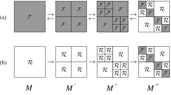
19, 21, 24, 26 in Algorithm 1). The recursive functionH-ApproxF (M ←M) is depicted in Fig. 5(a) for an example of an H-matrix with depth L = 2. Here, H-matrix M is converted to a block M
in F-format by converting R-blocks to F (M ← M) and coarsening the structure in the next two recursive steps (M ←M←M).
(a)
(b)
M
M
'M
''M
'''Figure 5. (a) Recursive function H-ApproxF (M → M) converting an F-block M to an H -matrixM. This procedure can also be implemented in the opposite order asF-ApproxH(M →M). (b) Recursive function H-ApproxR (M →M) converting an Rblock M to an H-matrix M. If H -matrixM has depth ofL, then L-step recursion (e.g.,M →M) and one final step (e.g., M→M) are needed for both cases (a) and (b). Here, to simplify the depiction, the depth of M is considered to beL= 2 which leads to 3 steps conversion.
IfZ∂V,∂V|r1×r2 is inH- orR-format, and the leaf level is reached for any ofZZZ∂V,V0 |r1×sorZZZV,∂V |s×r2
(lines 29–30, Algorithm 1), their product will be computed and stored as R or F. Here (line 30, Algorithm 1), the function FmtMulAdd (see Algorithm 2) performing formatted multiplication (at leaves) and addition [31] is called:
• If any of ZZZ∂V,V0 |r1×s orZZZV,∂V |s×r2 ∈ R (lines 2–9, Algorithm 2), the result of the multiplication
is stored as R. Hence, if ZZZ∂V,V0 |r1×s is H (line 3, Algorithm 2), recursive function HmulR (. . .)
truncation stepTrunRk+←Rk+k (. . . ) which is depicted in Fig. 7(a). This operation can be performed
by truncating the singular values of the matrix block stored in anR-format in Eq. (5) that can be done fast using reduced singular value decomposition (rSVD) [51, 7.1.1].
• If neither ZZZ∂V,V0 |r1×s nor ZZZV,∂V |s×r2 are in R-format (i.e., one of them is in F-format), the
multiplication result matrixZ ∂V,∂V|r1×r2 has to be stored inF-format (lines 10–18, Algorithm 2).
Algorithm 1 Multiplication and addition of H-matrices
Inputs: matricesZ∂V,∂V|r1×r2,ZZZ∂V,V0 |r1×s, and ZZZV,∂V |s×r2, clustersr1, r2 ∈∂V and s∈V.
Output: ZSVS=Z∂V,∂V ⊕(ZZZ∂V,V0 ⊗ZZZV,∂V )
1: MulAdd(Z∂V,∂V|∂V×∂V,ZZZ∂V,V0 |∂V×V,ZZZV,∂V |V×∂V,∂V,∂V,V)
2: function MulAdd(Z∂V,∂V|r1×r2,ZZZ∂V,V0 |r1×s,ZZZV,∂V |s×r2,r1,r2,s)
3: if (Z∂V,∂V|r1×r2 ∈ {H orR}) and(ZZZ0∂V,V|r1×s ∈ H) and(ZZZV,∂V |s×r2 ∈ H) then 4: for allri children of r1 do
5: for allrj children ofr2 do 6: for allsk children of sdo
7: if Z∂V,∂V|r1×r2 ∈ H then
8: MulAdd(Z∂V,∂V|ri×rj,ZZZ∂V,V0 |ri×sk,
ZZZV,∂V |sk×rj,ri, rj,sk) 9: else if Z∂V,∂V|r1×r2 ∈ R then
10: Z ∂V,∂V|ri×rj=GetPartR(Z∂V,∂V|r1×r2)
{GetPartR returns a part of matrixZ∂V,∂V inR-format corresponding to ri×rj child ofr1×r2}
11: MulAdd(Z ∂V,∂V|ri×rj,ZZZ∂V,V0 |ri×sk,
ZZZV,∂V |sk×rj,ri, rj,sk)
12: UpdatePartR(Z∂V,∂V|ri×rj, Z ∂V,∂V|ri×rj)
{UpdatePartR rewrites part of matrixZ∂V,∂V corresponding tori×rj withZ ∂V,∂V} 13: end if
14: end for 15: end for 16: end for
17: else if Z∂V,∂V|r1×r2 ∈ F then
18: if ZZZ∂V,V0 |r1×s∈ H then
19: H-ApproxF(F ←ZZZ0∂V,V|r1×s) {Fig. 5(a)}
20: else if ZZZ∂V,V0 |r1×s∈ Rthen
21: convertZZZ∂V,V0 |r1×s to F 22: end if
23: if ZZZV,∂V |s×r2 ∈ H then
24: H-ApproxF(F ←ZZZV,∂V |s×r2)
25: else if ZZZV,∂V |s×r2 ∈ Rthen
26: convertZZZV,∂V |s×r2 to F 27: end if
28: Z∂V,∂V|r1×r2+ =ZZZ∂V,V0 |r1×s×ZZZV,∂V|s×r2 {na¨ıve}
29: else if (Z∂V,∂V|r1×r2 ∈ {H orR}) and (ZZZ0∂V,V|r1×s∈ H/ orZZZV,∂V |s×r2 ∈ H/ ) then
30: FmtMulAdd(Z∂V,∂V|r1×r2,ZZZ∂V,V0 |r1×s,ZZZV,∂V |s×r2,r1,r2,s) 31: end if
Hence, for any ofZZZ∂V,V0 |r1×s orZZZV,∂V |s×r2 inH-format, they will be converted to the F usingH
-ApproxF (M ←M) in Fig. 5(a) and then na¨ıve multiplication is performed on the twoF-blocks.
Algorithm 2 Formatted multiplication (at leaves) and addition
Inputs: matricesZ∂V,∂V|r1×r2,ZZZ∂V,V0 |r1×s, and ZZZV,∂V |s×r2, clustersr1, r2 ∈TS and s∈TV.
Output: Z∂V,∂V|r1×r2 =Z∂V,∂V|r1×r2 ⊕(ZZZ∂V,V0 |r1×s⊗ZZZV,∂V |s×r2)
Require: (Z∂V,∂V|r1×r2 ∈ {H orR}) and(ZZZ0∂V,V|r1×s ∈ H/ orZZZV,∂V |s×r2 ∈ H/ )
1: function FmtMulAdd(Z∂V,∂V|r1×r2, ZZZ∂V,V0 |r1×s,ZZZV,∂V |s×r2,r1,r2,s)
FORMATTED MULTIPLICATION:
2: if (ZZZ∂V,V0 |r1×s ∈ R) or (ZZZV,∂V|s×r2 ∈ R) then{the result of multiplication Z∂V,∂V|r1×r2 is stored
asR}
3: if ZZZ∂V,V0 |r1×s∈ H then
4: Z ∂V,∂V|r1×r2 =HmulR(ZZZ∂V,V0 |r1×s, ZZZV,∂V |s×r2)
{Fig. 6}
5: else if ZZZV,∂V |s×r2 ∈ H then
6: Z ∂V,∂V|r1×r2 =RmulH(ZZZ∂V,V0 |r1×s, ZZZV,∂V |s×r2)
{Fig. 6}
7: else
8: Z ∂V,∂V|r1×r2 =ZZZ0∂V,V|r1×s·ZZZV,∂V |s×r2 9: end if
10: else if (ZZZ∂V,V0 |r1×s ∈ F) or (ZZZV,∂V|s×r2 ∈ F) then{Z∂V,∂V|r1×r2 is stored as F}
11: if ZZZ∂V,V0 |r1×s∈ H then
12: H-ApproxF(F ←ZZZ0∂V,V|r1×s) {Fig. 5(a)} 13: end if
14: if ZZZV,∂V |s×r2 ∈ H then
15: H-ApproxF(F ←ZZZV,∂V|s×r2) {Fig. 5(a)} 16: end if
17: Z∂V,∂V|r1×r2 =ZZZ0∂V,V|r1×s·ZZZV,∂V |s×r2 18: end if
FORMATTED ADDITION:
19: if (Z∂V,∂V|r1×r2 ∈ H) and (Z ∂V,∂V|r1×r2 ∈ F) then
20: H-ApproxF(Z ∂V,∂V|r1×r2 →Z∂V,∂V|r1×r2)
{Fig. 5(a)}
21: else if (Z∂V,∂V|r1×r2 ∈ H)and (Z ∂V,∂V|r1×r2 ∈ R) then
22: H-ApproxR(Z ∂V,∂V|r1×r2 →Z∂V,∂V|r1×r2)
{Fig. 5(b)}
23: end if
24: if Z∂V,∂V|r1×r2 ∈ H then
25: TrunHk+←Hk+k(Z∂V,∂V|r1×r2 , Z ∂V,∂V|r1×r2)
{Fig. 7(b)}
26: else{Z∂V,∂V|r1×r2 ∈ R}
27: if Z ∂V,∂V|r1×r2 ∈ F then
28: convertZ ∂V,∂V
|r1×r2 to R
29: end if
30: TrunRk+←Rk+k(Z∂V,∂V|r1×r2 , Z
∂V,∂V |r1×r2)
{Fig. 7(a)}
31: end if
M
21 12
=
M
21 M22
M
11 M12
21 12
=
Trun + ( M
11 11 + M12 21)
Trun + ( M
21 11 + M22 21)
Trun + ( M
11 12 + M12 22)
Trun + ( M
21 12 + M22 22)
=
M'
21 M
' 22
M'
11 M
' 12
M'
=
11
22
11
22
⊗ ⊗
Figure 6. Recursive functionRmulHX(R,H) performing formatted multiplication ofR- andH-blocks and storing the result inR-format. The recursive function HmulR (H,R) is defined similarly with an opposite order of operations. Here, to simplify the depiction, the depth ofH-matrix is considered to be
L= 1. In general,H-blocks of various depths occur.
k
+
k'
= k''
k
+
k
'
(b )
Z V , V|r1×r2 Z
' V , V
|r1×r2 Z V , V|r1×r2
+ k''
k
+
k
'
k
=
k'
(a )
Z V , V|r1×r2 Z
' V , V
|r1×r2
Z V , V∋ |r1×r2 ∋ ∋
∋ ∋ ∋
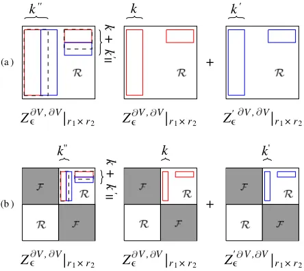
Figure 7. Procedures to re-compress the addition of two matrices. (a) Function TrunRk+←Rk+k(Z∂V,∂V|r1×r2, Z ∂V,∂V|r1×r2, τH) for addition and truncation of two matrices inR-format.
(b) Recursive functionTrunHk+←Hk+k(Z∂V,∂V|r1×r2, Z ∂V,∂V|r1×r2, τH) for addition and truncation of two
H-matrices. Again, to simplify the depiction, the depth ofH-matrices in (b) is considered to be L= 1. The resultant compressed blocks with revealed rankk are represented as dashed blocks.
As it is shown in Algorithm 2, after formatted multiplication the formatted addition is performed. Before adding the multiplication result matrix Z ∂V,∂V|r1×r2 to the matrix of Z∂V,∂V|r1×r2, the format
of Z∂V,∂V|r1×r2 is checked (lines 19–31, Algorithm 2):
• IfZ∂V,∂V|r1×r2 ∈ Hthe structure ofZ ∂V,∂V|r1×r2, which is in eitherF orRformat, is converted to
the hierarchical structure of Z∂V,∂V usingH-ApproxF (M → M) orH-ApproxR (M →M) in
Fig. 5, respectively (lines 20 and 22, Algorithm 2). After matching the structures, we add these two H-matrices and then compress the new createdH-matrix usingTrunHk+←Hk+k (. . . ) function (line 25,
re-compresses R-blocks from rank k+k to rank k using rSVD [51, 7.1.1] based on the predefined H-arithmetic toleranceτH in the newH-matrix.
• IfZ∂V,∂V|r1×r2 ∈ R, the structure ofZ
∂V,∂V
|r1×r2 is converted toRwhen it is inF-format (line 28,
Algorithm 2). Then, two R-blocks of Z∂V,∂V|r1×r2 and Z
∂V,∂V
|r1×r2 are added and compressed
through TrunRk+←Rk+k (. . . ) function with H-arithmetic tolerance τH in Fig. 7(a) (line 30, Algorithm 2).
5. MEMORY AND COMPUTATIONAL COMPLEXITY ANALYSIS FOR H-MATRIX SVS-EFIE
To derive the expressions for computational complexity and storage requirements, we define the sparsity constant [31] CspS×V for a given interaction tree TS×V, as
CspS×V := max ⎧ ⎪ ⎨ ⎪ ⎩ (a) max
r1∈TS, =0,...,L
#{s∈TV :r1×s∈ L(TS×V, )},
(b)
max
s∈TV, =0,...,L
#{r1 ∈TS :r1×s∈ L(TS×V, )} ⎫ ⎪ ⎬ ⎪ ⎭ (9)
where the term (a) in Eq. (9) is the maximum number of interaction blocks r1 ×s at the leaf level
associated with an observer cluster r1 ∈ TS, and the term (b) in Eq. (9) is the maximum number
of interaction blocks r1×s at the leaf level associated with a source cluster s∈ TV among all levels
= 0, . . . , Lof interaction treeTS×V. Here, L(TS×V, ) is the set of leaves at theth level, andL is the
number of levels of TS×V. The largest of these two counts is the sparsity constant CspS×V of TS×V.
As an example, for theH-matrix structure in Fig. 3 the number of interaction blocksr1×sassociated
with the observer cluster r1 =S1(3) at level 3 is:
#
s∈TV :S1(3)×s∈ L(TS×V,3)
= #
S(3)1 ×
V1(3), V
(3) 2 , V
(3) 3 , V
(3) 4
= 4 (10)
Also, at the same level = 3, the number of interaction blocks r1 ×s associated with the observer
cluster r1 =S3(3) is:
#
s∈TV :S3(3)×s∈ L(TS×V,3)
= #
S3(3)×
V1(3), V
(3) 2 , V
(3) 3 , V
(3) 4 , V
(3) 5 , V
(3) 6
= 6 (11)
After computing this counts for all observer clusters r1 ∈ TS in each level, the maximum number of
these counts among all four levels of this H-matrix is 6 for term (a) in Eq. (9). Analogously, for term (b) in Eq. (9), this maximum number among all source clusterss∈TV in each level of theH-matrix is 6. So, the sparsity constant CspS×V forH-matrix in Fig. 3 is maximum between the two counts (a) and
(b) in Eq. (9), which is 6.
Since in the interaction tree TV×S the domain and range are merely switched compared to the
interaction treeTS×V, and its sparsity constant is:
CspV×S =CspS×V =Csp (12)
To simplify the notation,M(·) will be used for asymptotic memory requirement inH-matrix format, while MR(·) and MF(·) are for the memory required by allR- and F-blocks, respectively.
5.1. Memory Complexity for SVS-EFIE H-Matrices
The memory usage to store volume-to-surfaceZZZ∂V,V0 and surface-to-volumeZZZV,∂V discretized operators
To compute the storage for the rectangular H-matrixZZZ∂V,V0 of the size P×3N, the storage ofR
-and F-blocks is analyzed, separately. Since all F-blocks exist only at the leaf level and the number of them scales linearly with the size of the matrix [31], the storage MF is estimated asO(n2min(N +P)),
withnmin×nmin being the size of the full leaf blocks.
On the other hand, rank deficientbthR-block of sizem()×n() at theth level is stored asABH
in Eq. (5), where matrix A is of size m()×kb∂V,V, and matrix BH is of size kb∂V,V ×n(). Therefore, its storage is kb∂V,V(m() +n()). Since, there are at most 2Csp interaction blocks at the th level
in the case of bisection based partitioning and considering sparsity constant definition in Eq. (9), the complexity to store all R-blocks forZZZ∂V,V0 can be approximated as
MRZZZ∂V,V 0
≤
LS
=0
2Cspk∂V,Vmax m() + LV
=0
2Cspkmax∂V,Vn(), (13)
where LS is the number of levels in TS and LV the number of levels in TV for theZZZ∂V,V0 interaction
tree TS×V, b = 1, . . . , NR, and kmax∂V,V is the maximum rank revealed (e.g., by ACA) among all NR
R-blocks of ZZZ∂V,V0 . Here, we assume kmax∂V,V to only weakly increase across the levels, hence, implying
quasi-dynamic simulation scenarios, in which the structure does not exceed several wavelengths in size. Since m() =P/2 and n() = 3N/2 are the sizes of the row and column of each R-block at the th level, respectively, andLS =O(logP) andLV =O(logN), Eq. (13) is simplified to
MRZZZ∂V,V0
≤Cspk∂V,Vmax
P
LS
=0
1 + 3N
LV
=0
1
=O(kmax∂V,VPlogP) +O(k∂V,Vmax NlogN). (14)
Therefore, the storageM(ZZZ∂V,V0 ) is dominated by the storage of itsR-blocks in Eq. (14)
MZZZ∂V,V0
=MR
Z ZZ∂V,V0
+MF
ZZZ∂V,V0
=O(kmax∂V,V(PlogP+NlogN)) +O(n2min(N +P))
=O(kmax∂V,VPlogP) +O(k∂V,Vmax NlogN),
(15)
where for simplicitykmax∂V,V is assumed to be ofO(nmin). Note that since theH-matrix structure ofZZZV,∂V
is a transpose ofZZZ∂V,V0 , asymptotically its storage is the same
MZZZV,∂V
=O(kmaxV,∂VPlogP) +O(kmaxV,∂VNlogN). (16)
ForP×P matrixZ∂V,∂V, the expression for the memory requirement can be derived by simplifying Eq. (15) for a squareH-matrix case:
M(Z∂V,∂V) =O(k∂V,∂Vmax PlogP). (17)
wherek∂V,∂Vmax is the maximum rank revealed (e.g., by ACA) among all R-blocks of ZZZ∂V,∂V .
5.2. Computational Complexity of H-GMRES Based Iterative Solver
The number of operations NMVP (complexity) of the MVP for an H-matrix can be bounded by the
memory required to store the H-matrix itself [32, Lemma 2.5]
NMVP(Z)≤ M(Z), Z ∈ {Z∂V,∂V, ZZZV,∂V , ZZZ∂V,V0 } (18)
Therefore, the computational complexity for H-GMRES based solver for SVS-EFIE is composed of three MVPs with the corresponding discretized integral operators:
NH-GMRES =Nit
NMVP(ZZZV,∂V ) +NMVP(ZZZ∂V,V0 ) +NMVP(Z∂V,∂V)
=Nit(O(kmaxPlogP) +O(kmaxNlogN)),
(19)
5.3. Computational Complexity of H-LU Based Direct Solver
As discussed in Section 4,H-LU based direct solver has three steps, the setup ofH-matrixZSVSinvolving
formatted multiplication and addition ofH-matricesZ∂V,∂V⊕ZZZ∂V,V0 ⊗ZV,∂V ,H-LU decomposition, and
backsubstitution. Below, we estimate computational complexity of these steps.
5.3.1. Formatted Multiplication ZZZ∂V,V0 ⊗ZZZV,∂V
As shown in Eq. (8), the complexity to setup ZSVS can be estimated through formatted multiplication
and addition of H-matrices. To simplify the analysis, at first the truncation functions TrunHk+←Hk+k
(. . . ) andTrunRk+←Rk+k (. . . ) in Algorithm 2 will be considered as a simple copying of the data without
any re-compression, sok =k+k in Fig. 7. For this scenario, the formatted multiplication of two sub-blocksZZZ∂V,V0 |r1×s⊗ZZZV,∂V |s×r2 in Algorithm 1, line 30 (see also lines 4 and 6 of Algorithm 2) becomes
the exact multiplication ZZZ∂V,V0 |r1×s×ZZZV,∂V |s×r2 in H-matrix format.
So, in Algorithm 2, each leaf block r1 ×r2 at the jth level resulting from the multiplication
ZZZ∂V,V0 |r1×s×ZZZV,∂V |s×r2 is performed with
Z
ZZ∂V,V0 |r1×s×ZZZV,∂V |s×r2
|r1×r2 =
ι
=0
s∈ U(r1×r2,)
ˆ
Z Z
Z∂V,V0 |r1×s×ZZZˆ
V,∂V |s×r2
, (20)
whereι∈[0, L] whichL is the depth ofH-matrices ZZZ∂V,V0 andZZZV,∂V . Also,
U(r1×r2, ) =
s∈TV():{R(r1)×s∈TS×V and s×R(r2)∈ L(TV×S)}
or{R(r1)×s∈ L(TS×V)and s×R(r2)∈TV×S}
,
(21)
and
V =
·
=0,...,ι
·
s∈ U(r1×r2,)
s. (22)
In Eq. (21), R(r1) is the relative of clusterr1 (ancestor ( < j), self (=j), or descendant ( > j)) at
th level, and L(TV×S) is a leaf of the TV×S interaction tree. Hence, in Eq. (20) sub-block ˆZZZ∂V,V0 |r1×s,
or sub-block ˆZZZV,∂V |s×r2, or both are in the leaf level of the corresponding interaction tree and are stored
asR- or F-blocks.
SinceF-blocks have the size of at mostnmin×nmin,H-matrix-matrix product with them requires
nmin MVPs, while the exact H-matrix-matrix product with an R-block involves k MVPs. Therefore,
to compute ZZZ∂V,V0 |r1×s×ZZZV,∂V |s×r2 in Eq. (20) at any level will require at most max (kmax, nmin)
MVPs, where kmax is the maximum rank revealed forZZZ∂V,V0 and ZZZV,∂V . Without loss of generality if
kmax ≥nmin, the complexity N to compute the product of sub-blocksZZZ∂V,V0 |r1×s and ZZZV,∂V |s×r2 can
be estimated as
NZZZ∂V,V0 |r1×s∈L(TS×V,)×ZZZV,∂V |s×r2∈(TV×S,)
≤k∂V,Vmax NMVP(ZZZV,∂V |s×r2∈(TV×S,))
(18)
≤ k∂V,Vmax M(ZV,∂V |s×r2∈(TV×S,)), kmax∂V,V ≥nmin
(23) Similarly,
N ZZZ∂V,V0 |r1×s∈(TS×V,)×ZZZV,∂V |s×r2∈L(TV×S,)
≤kV,∂Vmax M(ZZZ∂V,V0 |r1×s∈(TS×V,)), kV,∂Vmax ≥nmin (24)
The overall complexity to multiplyZZZ∂V,V0 andZZZV,∂V can be calculated by analyzing the interaction
r1×r2∈ L(TS×S, j) at the jth level of Eq. (20), j= 1, . . . , LS, the complexity estimate is
N(ZZZ∂V,V0 ×ZZZV,∂V )≤ LS
j=0
r1×r2∈L(TS×S,j)
×
L
=0
s∈U(r1×r2,)
N
ˆ
ZZZ∂V,V0 |r1×s×ZZZˆ
V,∂V |s×r2
(25)
whereLis the depth ofH-matricesZZZ∂V,V0 andZZZV,∂V . By substituting Eqs. (23) and (24) into Eq. (25),
it can be written as:
N(ZZZ∂V,V0 ×ZZZV,∂V )≤ LS
j=0
r1×r2∈L(TS×S,j) L
=0
s∈U(r1×r2,)
kV,∂Vmax M(ZZZ∂V,V0 |r1×s) +k∂V,Vmax M(ZZZV,∂V |s×r2)
,
(26) Considering the definition in Eq. (22) for the union of all the volume clusters s contributing to formation of the destination blockr1×r2the operation count
L
=0
s∈U(r1×r2,)(kmaxV,∂VM(ZZZ∂V,V0 |r1×s)+ kmax∂V,VM(ZZZV,∂V|s×r2)) in the summation over the volume clusters s in Eq. (26) can be simplified by
considering the root cluster V containing all volume basis/testing functions, yielding
N(ZZZ∂V,V0 ×ZZZV,∂V )≤ LS
j=0
r1×r2∈L(TS×S,j)
kV,∂Vmax M(ZZZ∂V,V0 |r1×V) +k∂V,Vmax M(ZZZV,∂V |V×r2)
(27)
On the other hand, for each level j, the total number of leaf blocks r1 ×r2 ∈ L(TS×S, j) in
the resultant interaction tree TS×S is bounded by 2jCspS×S in case of bisection based partitioning
and considering sparsity constant definition in Eq. (9). Here, 2j is the total number of observer clusters r1 or source clusters r2 at the jth level of interaction tree TS×S. Therefore, in Eq. (27) the
number of operations (estimated via memory use) in summationsr1×r2∈L(T
S×S,j)M(ZZZ∂V,V0 |r1×V) and
r1×r2∈L(TS×S,j)M(ZZZV,∂V |V×r2) required for computation of the resultant leaf clustersr1×r2at levelj
can be replaced by the operation countCspS×S(M(ZZZ∂V,V0 |∂V×V) +M(ZV,∂V |∂V×V)) over the root cluster
∂V containing all the surface RWG basis/testing functions. So, Eq. (27) can be rewritten as:
N(ZZZ∂V,V0 ×ZZZV,∂V )≤ LS
j=0
CspS×S
kmaxV,∂VM(ZZZ∂V,V0 |∂V×V) +k∂V,Vmax M(ZZZV,∂V |V×∂V)
(28)
Here, M(ZZZ∂V,V0 |∂V×V) and M(ZZZV,∂V|V×∂V) can simply be replaced by M(ZZZ∂V,V0 ) and M(ZV,∂V )
denoting the memory use for storage of the H-matrices ZZZ∂V,V0 and ZZZV,∂V , respectively. Then, by
recalling that the depth of the surface tree isLS =O(logP) and introducing the maximum rankkmax
for blocks of eitherZZZ∂V,V0 orZZZV,∂V (i.e., kmax= max (kmax∂V,V, kV,∂Vmax )), Eq. (28) becomes
N(Z∂V,V0 ×ZZZV,∂V )≤LSCspS×Skmax
M(ZV,∂V
) +M(Z∂V,V0 )
. (29)
Recalling the estimates for memory use Eqs. (15) and (16) we finally get the estimate for operation count in theexact multiplication of theH-matrices
N(ZZZ∂V,V0 ×ZZZV,∂V ) =O
k2maxPlog2P
+Okmax2 NlogNlogP
. (30)
Note that the formatted multiplicationZZZ∂V,V0 ⊗ZZZV,∂V requires the truncation based on the prescribed
H-arithmetic toleranceτHof small singular values resulting from addition of theR-blocks. For that, the
rSVD with the complexity of O(n() +m())k2+O(k3) [51, 7.1.1] is used throughout the Algorithm 2 leaving the complexity estimate of Eq. (30) correct for the formatted multiplication as well (i.e., N(ZZZ∂V,V0 ×ZZZV,∂V ) N(ZZZ∂V,V0 ⊗ZZZV,∂V )) provided kmax is relatively small compared to P and N
5.3.2. Formatted AdditionZZZ∂V,∂V ⊕(ZZZ∂V,V0 ⊗ZZZV,∂V )
Next, the complexity of the formatted addition of twoH-matrices of the sizeP×Prequired to formZSVS
by addingZ∂V,∂V and the result ofZZZ∂V,V0 ⊗ZZZV,∂V in Eq. (8) has to be considered. For formatted addition
of the squareH-matrices, the estimate for number of operations isO(k2maxPlogP)+O(k3maxP) [31]. The
total complexity for setting up theZSVSis composed of the complexity of the formatted multiplication
in Eq. (30) and the formatted addition as
N(ZSVS) =O
kmax2 Plog2P
+Ok2maxNlogNlogP
+O(kmax3 P) (31)
One can see that for the problems of electrically moderate sizes with bounded rank, the complexity for setting up the ZSVS is dominated by the complexity of the formatted multiplication in Eq. (30).
5.3.3. H-LU Decomposition and Back Substitution
To solve the matrix equations, H-LU decomposition and back substitution are applied to ZSVS. Since
ZSVSis a squareH-matrix of the sizeP×P, the time complexity for theH-LU decomposition and back
substitution areO(k3maxPlog2P) and O(kmax3 PlogP), respectively [31].
6. NUMERICAL RESULTS
To validate the accuracy of theH-matrix SVS-EFIE solver, we performed comparison of its numerical solutions against the analytic Mie series [52] and the results obtained using FEKO commercial solver [53] for several scattering problems. The performance of the SVS-EFIE solver for the timing and memory requirements is shown to corroborate the asymptotic complexities derived in Section 5. In all the numerical results, we considered the tolerance for H-matrix compression τH to be the same as the
truncation tolerance of the ACA algorithm τACA. So, for brevity τ = τACA = τH is used throughout
Section 6. The optimal values of the admissibility criterion η and leafsize nmin are usually problem
dependent and chosen empirically. The H-matrix parameters in the paper are the optimized values forη ={1,2,3,4,5} and nmin ={8,16,32,64} sets in all numerical examples. It was observed that all
combinations of these parameters are working well for the proposed solver. However, to balance between memory use and CPU time we run the numerical example for different parameters and empirically find thatη= 4 andnmin = 16 provide better time and memory performance for certain numerical examples
of this paper.
6.1. Dielectric Sphere
In the first example, we consider scattering on a dielectric sphere of radius R = 0.1 m and relative dielectric permittivity = 1.5 excited by a radial dipole with the dipole momentI= 1[A·m].
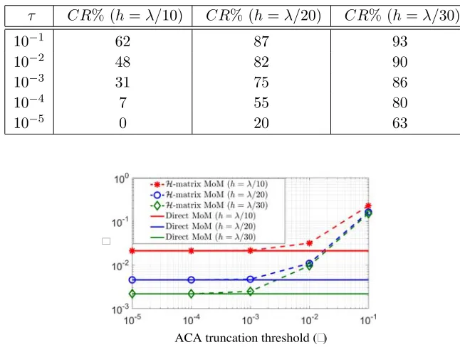
To demonstrate the behavior of the error inH-matrix accelerated MoM solution of SVS-EFIE and its reduction with the decrease of ACA truncation threshold τ, we consider dielectric sphere excitation by a z-directed electric dipole at 3 GHz situated above the north pole of the sphere 0.4 m away from the origin. The behavior of the average relative error (δ) of both H-matrix accelerated MoM solution and direct MoM solution of the SVS-EFIE [40] with respect to the Mie series solution is depicted as a function of τ in Fig. 8 for three different mesh densities, h = λ/10, λ/20, and λ/30, h being the characteristic size of mesh elements. The results demonstrate thatH-matrix accelerated MoM solution with τ ≤ 10−3 does not produce any substantial increase in accuracy compared to the direct MoM
solution. On the other hand, the compression ratio (CR) of the overall MoM memory use in SVS-EFIE is shown for different τ in Table 1, where
CR =
1− Mem. H-matrix SVS-EFIE Mem. direct MoM SVS-EFIE [40]
×100%. (32)
Table 1. Memory compression ratio (32) for theH-matrix accelerated MoM solution of the SVS-EFIE for the dielectric sphere excitation problem with different mesh densities (h =λ/10, λ/20, and λ/30).
τ CR% (h=λ/10) CR% (h=λ/20) CR% (h=λ/30)
10−1 62 87 93
10−2 48 82 90
10−3 31 75 86
10−4 7 55 80
10−5 0 20 63
ACA truncation threshold (τ)
τ
Figure 8. Average relative error δ of both H-matrix accelerated MoM solution for dielectric sphere excitation problem with different mesh densities (h =λ/10, λ/20, andλ/30) with respect to the Mie series solution as a function of ACA truncation tolerance τ. The error in the direct MoM solution of SVS-EFIE [40] is shown for reference.
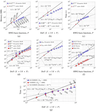
To analyze theH-matrix acceleration performance for MoM solution with large number of degrees of freedom (DoF), we examine the memory usage by theH-matrices and CPU time used for pertinentH -matrix operations in comparison with those in the direct MoM solution [40]. For this study, the dielectric sphere with mesh density h=λ/10 over the frequency range from 4 GHz to 10 GHz is considered.
In Fig. 9(a), the memory usage forZ∂V,∂V is demonstrated as a function of number of RWG basis functions P. Its H-matrix MoM scaling behaves as O(PlogP) confirming the theoretical estimates in Eq. (17). In addition, the memory requirement of ZZZ∂V,V0 and ZZZV,∂V is also depicted in Fig. 9(b)
with respect to the total number of surface and volume DoFs X = 3N +P. It can be seen that the numerically observed memory scaling ofO(NlogN) +O(PlogP) for H-matrix MoM confirms the theoretical estimates in Eqs. (15) and (16).
Next, in Figs. 9(c) and (d), the time required to fill the compressed H-matrices is plotted. Fig. 9(c) shows the time to fill Z∂V,∂V that behaves as O(PlogP) for H-matrix solver. Also, the CPU time to fill ZZZ∂V,V0 and ZZZV,∂V is plotted as a function of total number of surface and volume
DoFs X = 3N +P in Fig. 9(d). One can observe fill time complexities of O(NlogN) +O(PlogP) which is of the same order as the memory use complexity in Eqs. (15) and (16). In addition, the set up time for creating ZSVS as a part of the H-LU direct method is depicted in Fig. 9(e) with the
complexity of O(NlogNlogP) +O(Plog2P) which confirms the theoretical analysis in Eq. (31). The time complexities for H-LU decomposition and back-substitution are also plotted in Fig. 9(f) with scaling ofO(Plog2P) and O(PlogP), respectively [31].
For the same scattering problem, the computational time using H-GMRES iterative method is plotted in Fig. 9(g). In the first study, the number of iterations is fixed to Nit = 1000 and the time
is plotted in blue triangles as a function of number of DoFs leading to Nit(O(NlogN) +O(PlogP))
iterative solver tolerance is set to 10−6, and the solution time is depicted in red crosses in the same figure.
In this study, the dielectric sphere having = 1.5 has a relatively small electrical radius ranging from R = 1.6λ to R = 4λ in the considered frequency range from 4 GHz to 10 GHz. Therefore, the maximum rank will be approximately constant for all H-matrices [50] in the entire frequency range. It can be seen from Figs. 9(a)–(f) that the memory requirement and CPU time scale according to the constant rank assumption.
Memory (MB)
RWG basis functions, P
3G Hz 4G
Hz 5G Hz
4 G
H z 5
G H
z 6
G H
z 7
G H
z 8
G H
z 9
G H
z 10
GH z
DoF (X = 3N + P)
Time
(s
)
RWG basis functions, P
Do F (X = 3N + P)
(d)
Do F (X = 3N + P)
(e)
RWG basis functions, P
(f)
Time
(s
)
DoF (X = 3N + P)
(g)
Nit
= 440
555 730
1050 1330 2120
2800
(a) (b) (c)
Figure 9. Scaling behavior of both H-matrix (dashed lines) and direct (solid lines) MoM SVS-EFIE for the dielectric sphere with mesh density h=λ/10 across the frequency range from 4 GHz to 10 GHz. (a) Memory for Z∂V,∂V. (b) Memory forZZZ∂V,V0 and ZZZV,∂V . (c) Set up time for Z∂V,∂V. (d) Set up
time for Z∂V,V0 andZZZV,∂V . (e) Set up time forZSVS as a part of H-LU-based direct solver. (f) Solution