Classical Power and Energy Relations for Macroscopic Dipolar
Continua Derived from the Microscopic Maxwell Equations
Arthur D. Yaghjian*
Abstract—Positive semi-definite expressions for the time-domain macroscopic energy density in passive, spatially nondispersive, dipolar continua are derived from the underlying microscopic Maxwell equations satisfied by classical models of discrete bound dipolar molecules or inclusions of the material or metamaterial continua. The microscopic derivation reveals two distinct positive semi-definite macroscopic energy expressions, one that applies to diamagnetic continua (induced magnetic dipole moments) and another that applies to paramagnetic continua (alignment of “permanent” magnetic dipole moments), which includes ferro(i)magnetic and antiferromagnetic materials. The diamagnetic dipoles are “unconditionally passive” in that their Amperian (circulating electric current) magnetic dipole moments are zero in the absence of applied fields. The analysis of paramagnetic continua, whose magnetization is caused by the alignment of randomly oriented “permanent” Amperian magnetic dipole moments that dominate any induced diamagnetic magnetization, is greatly simplified by first proving that the microscopic power equations for rotating “permanent” Amperian magnetic dipoles (which are shown to not satisfy unconditional passivity) reduce effectively to the same power equations obeyed by rotating unconditionally passive magnetic-charge magnetic dipoles. The difference between the macroscopic paramagnetic and diamagnetic energy expressions is equal to a “hidden energy” that parallels the hidden momentum often attributed to Amperian magnetic dipoles. The microscopic derivation reveals that this hidden energy is drawn from the reservoir of inductive energy in the initial paramagnetic microscopic Amperian magnetic dipole moments. The macroscopic, positive semi-definite, time-domain energy expressions are applied to lossless bianisotropic media to determine the inequalities obeyed by the frequency-domain bianisotropic constitutive parameters. Subtleties associated with the causality as well as the group and energy-transport velocities for diamagnetic media are discussed in view of the diamagnetic inequalities.
1. INTRODUCTION
As a way of introducing the motivation for and purpose of this paper, begin with the familiar Maxwell macroscopic equations that hold in dipolar continua (without current J) to obtain the macroscopic Poynting theorem as1
−
S
ˆ
n·[E(r, t)×H(r, t)]dS =
V
∂D(r, t)
∂t ·E(r, t) +
∂B(r, t)
∂t ·H(r, t)
dV (2)
Received 19 August 2016, Accepted 24 October 2016, Scheduled 7 November 2016
* Corresponding author: Arthur D. Yaghjian ([email protected]).
The author is with Electromagnetics Research Consultant, 115 Wright Road, Concord, MA 01742, USA.
1 In reading Poynting’s original 1884 paper, one finds that he wrote his theorem in the form (using modern notation and SI units
with displacement current written as∂D/∂tinstead of∂E/∂tandμ∂H/∂twritten as∂B/∂t)
V
∂D
∂t ·Ev+ ∂B
∂t ·H+J·Ev+
J+∂D
∂t
×B·vdV =−
S
ˆn·(E×H)dS (1)
whereEv=E+v×Bandvis the velocity of the “matter” [1, eq. (7)]. This is not too surprising since Poynting references Maxwell’s
with
D=0E+P, B=μ0(H+M) (3)
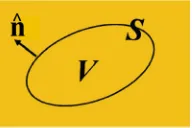
where (E,D) and (B,H) are the macroscopic electric and magnetic fields, respectively, PandMare the macroscopic electric and magnetic dipolarization densities, respectively, and0andμ0are the free-space permittivity and permeability, respectively. (The term “macroscopic” is used throughout to designate electromagnetic fields and sources averaged over macroscopic volumes that contain a large number of discrete dipolar molecules or inclusions while having dimensions much smaller than the minimum temporal and spatial wavelengths in free-space and in the continuum. An electromagnetic “dipolar continuum” or just “continuum” is used throughout to refer to a medium in which fields and sources obey the traditional Maxwell dipolarization equations; see Eq. (28) or (46). We will later find it useful to distinguish between “ideal” and “macroscopic” continua.) The unit normalnˆ to the closed surface
S points out of its volumeV so that the left-hand side (and thus the right-hand side) of Eq. (2) is (as will be proven later) equal to the instantaneous electromagnetic power flow entering the volumeV; see Fig. 1. Integrating Eq. (2) from timet0when the macroscopic fields are zero to the present timetgives a macroscopic electromagnetic energy density on the right-hand side of Eq. (2) equal to
t
t0
∂D(r, t)
∂t ·E(r, t
) + ∂B(r, t)
∂t ·H(r, t
)dt. (4)
If it is assumed that the macroscopic electromagnetic energy in a passive polarized continuum is at least as great as the energy of the sameE andHfields produced in a vacuum, then this vacuum energy density is (0|E|2+μ0|H|2)/2 and Eq. (4) yields the inequality
t
t0
∂D(r, t)
∂t ·E(r, t
) + ∂B(r, t)
∂t ·H(r, t
)dt ≥ 1
2 0|E(r, t)| 2+μ
0|H(r, t)|2
(5)
or simply
t
t0
∂P(r, t)
∂t ·E(r, t ) +μ
0∂
M(r, t)
∂t ·H(r, t
)dt ≥0. (6)
If, on the other hand, one takes the view that all known magnetization is produced by Amperian magnetic dipoles (circulating electric current) and thusEandBare the primary fields, then the vacuum energy density is (0|E|2+|B|2/μ0)/2 and Eq. (4) yields instead of Eqs. (5) and (6)
t
t0
∂D(r, t)
∂t ·E(r, t
) +∂B(r, t)
∂t ·H(r, t
)dt ≥ 1
2
0|E(r, t)|2+ 1
μ0|
B(r, t)|2
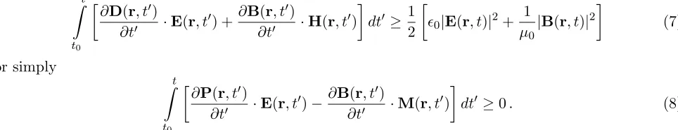
(7)
or simply
t
t0
∂P(r, t)
∂t ·E(r, t
)−∂B(r, t)
∂t ·M(r, t
)dt ≥0. (8)
Although it is often argued that Eq. (6) is the correct inequality for passive continua [4–6], [7, p. 81], in fact, neither one of the inequalities in Eq. (6) or (8) are universally valid because the simple hypothetical example of a passive material with constitutive relations D =E and B =μHwith real constant permittivity and permeability μover the operational bandwidth reveals from Eq. (6) that
≥0, μ≥μ0 (9) and from Eq. (8) that
Figure 1. VolumeV with surfaceS in dipolar continua with macroscopic polarization densitiesPand M.
conditions and without assuming any particular constitutive parameters, Eqs. (6) and (8) apply to paramagnetic and diamagnetic dipolar continua, respectively.
To prove these positive semi-definite time-domain inequalities in Eqs. (6) and (8), the macroscopic Maxwell equations and Poynting theorem are systematically related to the more fundamental microscopic Maxwell equations and Poynting theorem from which their macroscopic counterparts are derived. Diamagnetic material is defined simply as material with Amperian magnetization produced by molecules or inclusions that have no permanent magnetic dipole moments, only induced magnetic dipole moments. Paramagnetic material, a term that includes ferro(i)magnetic and antiferromagnetic material [8, chs. 11 and 12],is defined simply as material with magnetization produced by the alignment of “permanent” (sometimes called “intrinsic”) Amperian magnetic dipole moments of molecules or inclusions that dominate any induced diamagnetic magnetization.2 Notably, the detailed microscopic derivation using classical models of electric and magnetic dipoles reveals that the difference between the integrals of the power densities in Eqs. (6) and (8), what can be called the macroscopic hidden energy, is drawn from the reservoir of inductive energy in the permanent (initial paramagnetic) microscopic Amperian magnetic dipoles. (The term “permanent” does not imply that the value of the initial current and magnitude of the magnetic dipole moment cannot change slightly as the magnetic dipole rotates in an external field.)
Besides the Introduction and Conclusion, the paper contains six other main sections:
In Section 2, the mathematically rigorous vector-scalar potential solution is given to Maxwell’s differential equations for microscopic electric current and charge density. From these equations, it is established that the microscopic Poynting vector integrated over a closed surface in free space equals the total instantaneous power crossing that free-space surface. It is further shown that, in passive materials, the energy supplied by the fields to the microscopic charge carriers from the time the external fields are first applied is always positive semi-definite (nonnegative).
In Section 3, Maxwell’s continuum equations are derived from the microscopic equations of Section 2 for an ideal continuum, defined by infinitesimal subvolumes of electric and magnetic dipolarization that are continuous, and a straightforward proof is given that these same Maxwell equations describe the macroscopic dipolarization obtained from averaging the sources and fields of classical models of discrete electric and magnetic dipoles. It is shown that a requirement for the equivalence of the ideal and macroscopic continua equations is that the surfaces of the macroscopic averaging volumes lie in free space and not cut through the discrete dipoles.
In Section 4, the conditions are found (namely that the continuum is effectively spatially nondispersive) for the macroscopic continuum Poynting vector integrated over a closed surface to equal the instantaneous power flow across that closed surface.
Section 5 begins with a derivation of expressions for macroscopic continua energy densities in terms of the microscopic energy densities. It is determined that, under sufficient conditions that are designated by the term “unconditionally passive”, one of these energy-density expressions remains positive semi-definite for diamagnetic media, and a second different energy-density expression remains positive semi-definite for paramagnetic media.
In Section 6, the important positive semi-definite energy-density expressions for macroscopic continua are summarized for paramagnetic and diamagnetic continua and it is shown that the difference between these two energy densities equals a “hidden energy” extracted from the energy in the
2 These fundamental definitions of diamagnetism and paramagnetism differ from the more common definitions as materials (or
“permanent” Amperian microscopic magnetic dipole moments that align to produce the paramagnetic dipolarization.
In Section 7, the positive semi-definite time-domain inequalities of Section 6 are applied to paramagnetic and diamagnetic bianisotropic continua to derive inequalities satisfied by lossless frequency-domain bianisotropic constitutive parameters. Lastly, subtleties associated with diamagnetic continua are discussed, namely, the causality of diamagnetic permeability as well as the group and energy-transport velocities in lossless diamagnetic media.
We employ a classical analysis of macroscopic dipolar continua in which no attempt is made to determine the detailed quantum nature of the polarizations and fields of atoms and molecules. It is assumed, as in most texts on the electromagnetic fields and equations of polarized media, that since most materials below optical frequencies and dipolar metamaterials well below bandgap frequencies are adequately described by the classical Maxwell macroscopic equations for a dipolar continuum, the microscopic dipoles producing the macroscopic dipolarization can be adequately modeled pragmatically by classical electric-charge electric dipoles and Amperian-current magnetic dipoles, irrespective of their actual quantum origin.
There are several reasons for determining nonnegative macroscopic energies from the microscopic Maxwell equations for classical diamagnetic and paramagnetic dipolar continua. First, it is one of the remaining unresolved problems in classical electromagnetic theory even though the problem is relatively easy to state: given a volume of a macroscopic continuum satisfying Maxwell’s dipolar equations and illuminated by external fields, are there macroscopic polarization energy densities that never become negative for all times after an initial time when the macroscopic fields and polarizations are zero. Nonnegative energy expressions provide a means for determining realistic physical limitations, such as the upper bounds on the bandwidth and gain of antennas or the lower bounds on antenna quality factors. Valuable inequalities satisfied by bulk constitutive parameters as well as by the group and energy transport velocities in materials and metamaterials can be obtained from nonnegative macroscopic energy expressions. Also, knowing the sufficient conditions for the validity of the nonnegative macroscopic energy expressions lends insight into the development and utilization of materials and metamaterials that may not be subject to the restrictions imposed by these expressions.
2. MAXWELL’S EQUATIONS FOR MICROSCOPIC ELECTRIC CHARGE AND CURRENT
We assume that we are dealing with macroscopic continua whose molecules or inclusions can be modeled by classical microscopic electric charge and current whose fields can be adequately described by the following Maxwell differential equations in SI (mksA) units
∇ ×e(r, t) + ∂b(r, t)
∂t = 0 (11a)
1
μ0∇ ×
b(r, t)−0∂ e(r, t)
∂t =j(r, t) (11b)
∇ ·b(r, t) = 0 (11c)
0∇ ·e(r, t) =(r, t) (11d)
d is given byd=0eand the microscopic secondary magnetic field h is given byh=b/μ0.3
The rigorous vector-scalar potential solution to Maxwell’s Equations (11) in the frequency domain (with e−iωt time dependence) is given by [12, sec. 2.3.6]
bω(r) = ∇ ×aω(r) (12a)
eω(r) = iωaω(r)− ∇ψω(r) (12b)
with the vector and scalar potentials determined from the expressions
aω(r) =μ0lim
δ→0
V−Vδ
jω(r)G(|r−r|)dV (13a)
ψω(r) = 1
0 lim
δ→0
V−Vδ
ω(r)G(|r−r|)dV (13b)
and the scalar Green’s function given by
G(|r−r|) = e
ik0|r−r|
4π|r−r|, k0=ω
√
μ00. (13c)
The limits before the integrals of Eq. (13) are rigorously required to isolate the singularity in the Green’s function at r =rfrom the volume integration by a “principal volume” Vδ (with maximum dimension
δ) to allow rigorous differentiation of the potentials to obtain the fields in Eq. (12) [12, sec. 2.3.6], [13].
2.1. Poynting’s Theorem for Microscopic Electric Charge and Current
Let the microscopic charge and current be confined to a region of finite extent so that they can be enclosed by a volume V whose surface S lies in free space. Then the instantaneous power Pje(t) supplied by the fields to the charge-current within V is simply
Pje(t) =
V
j(r, t)·e(r, t)dV . (14)
This is proven from the Lorentz force on a volume charge density v moving with velocity v, namely
dF =v(e+v×b)dV with dP =v·dF =vv·edV =j·edV.4 (Thus, the magnetic field does not impart energy to the charge carriers.) With the help of Eqs. (11a) and (11b), the power in Eq. (14) can be recast in the form of the microscopic Poynting theorem
Pje(t) =
V
j·edV =−
V
∇ ·(e×b/μ0) + 1 2
∂ ∂t
0|e|2+|b|2/μ0
dV (15)
or by means of the divergence theorem as
S
ˆ
n·(e×b/μ0)dS =−
V
j·edV −1
2
d dt
V
0|e|2+|b|2/μ0
dV (16)
withnˆ denoting the unit normal to S pointing out of the volume V.
As any one of an infinite number of test examples to which Eq. (16) can be applied, suppose that the volume V contains a charged capacitor C that is shorted at t = 0 through an inductor L. Even if the capacitor, the inductor, and the wires are lossless conductors, this LC circuit will not oscillate
3 For metamaterial inclusions with microscopic polarization densitiespandm, the currentjin Eq. (11) would include∂p/∂t+∇ ×m,
and the chargewould include−∇ ·p. Thus, the main results of this paper are applicable to these metamaterials as well within the bandwidths that they behave as dipolar continua [10, 11], provided either paramagnetism or diamagnetism dominates the macroscopic magnetization produced by the inclusions. For example, metal-dielectric inclusions in metamaterial-array continua would be described by the electric-dipole/diamagnetic energy expressions.
4 The Lorentz force ondV is exerted by the fields of all sources except the fields of dV itself. However, the self-fields of an
forever because it will radiate. At the timet=T, assume that the radiation has practically reduced the oscillations of the RL circuit to zero and that the surfaceS is chosen far enough away that the radiated fields have not reached S at the time T. Then Eq. (16) becomes after integrating over time from 0− to
T
1 2
V
0|e(r,0−)|2dV =
T
0−
V
j(r, t)·e(r, t)dV dt+1 2
V
0|e(r,T)|2+|b(r,T)|2/μ0
dV (17)
where 0− denotes the time just beforet= 0. The left-hand side of Eq. (17) is equal to the electrostatic energy stored initially by the capacitor, a result that is rigorously proven from the electrostatic equations under a quasi-static charging of the capacitor plates. As explained above, the first integral on the right-hand side of Eq. (17) is the energy supplied by the fields to the charge carriers of the current. (It is zero for a stationary lossless conductor and greater than zero for a lossy conductor.) Therefore, the second integral on the right-hand side of Eq. (17) is an additional energy required by conservation of energy. In other words, V[0|e(r, t)|2+|b(r, t)|2/μ0]dV /2 is the free-space energy stored in the electromagnetic fields in the volume V not only for statics but also for time dependent fields at each instant of timet. With this established, we see that the right hand side of Eq. (16), and thus the left-hand side of Eq. (16), is the time rate of change of the total energy leaving the volume V. In particular, the integral of the time-dependent microscopic Poynting vector, that is,nˆ·[e(r, t)×b(r, t)/μ0], over a closed surfaceS lying in free space is the total instantaneous electromagnetic power leaving that closed surface. Alternatively, the total instantaneous electromagnetic powerP(t) entering a closed surfaceS that lies in free space is given by
P(t) = −
S
ˆ
n·[e(r, t)×b(r, t)/μ0]dS
=
V
j(r, t)·e(r, t)dV +1 2
d dt
V
0|e(r, t)|2+|b(r, t)|2/μ0
dV . (18)
This result is true whether or not the microscopic charge-current inside S forms polarized material, providedS lies in free space outside the material. However, this result does not imply thatˆn·(e×b/μ0) is necessarily the instantaneous free-space power flow per unit area in the direction ofn. In other words,ˆ the integral ofˆn·(e×b/μ0) over an open free-space surface does not necessarily equal the electromagnetic power that flows across that open surface.
2.1.1. Energy Supplied to the Charge Carriers
The instantaneous power supplied by the electromagnetic fields to the charge carriers (usually electrons and positively charged nuclei) producing the microscopic charge and current (,j) that generate the fieldse and b under consideration in V is given in Eq. (14). Expressing Pje(t) as the time derivative of an energyWje(t), that is,Pje(t) =dWje(t)/dt, and integrating the power in Eq. (14) from an initial timet0 in the past to the present timet, we obtain
Wje(t)−Wje(t0) =
t
t0
V
j(r, t)·e(r, t)dV dt. (19)
charge carriers.5 These other forces are fundamentally electromagnetic forces from the fields of the host material, namely from the fields of the atomic and molecular charges other than the charge carriers that produceeandb. They are the forces, for example, involved in the conversion of the kinetic energy of the charge carriers into heat (out-of-band energy), or into the kinetic-potential-heat energy of the springs in a compressed-spring model of electric dipoles, or into the kinetic-potential-heat energy of expandable conducting wires in a wire-loop model of Amperian magnetic dipoles.
If the macroscopic continuum is passive in that (i) there is negligible initial kinetic energy of the bound charge carriers within the operational bandwidth (that is, negligible in-band initial kinetic energy) that can be decreased, (ii) there is negligible in-band net energy transfer from the host material to the charge carriers (that is, in-band energy cannot travel through the host material, except by means ofeandb, from one region of the continuum to the other), and (iii) there are no auxiliary sources (such as chemical reactions changing the e and b fields so as to add to the energy of the charge carriers, or initial kinetic-potential energy stored in the springs of a compressed-spring model of electric dipoles, or in expandable conducting wires of “permanent” Amperian magnetic dipoles)that can release energy upon excitation by applied fields to serve as an active source of internal energy increasing the energy of the charge carriers, thenWje(t)−Wje(t0)≥0. In other words, if there is no initial in-band mechanical energy, and no internal active sources of energy, and no nonlocal transfer of in-band mechanical energy, then the material is passive such that Wje(t)−Wje(t0) ≥0. Choosing the arbitrary, constant initial energyWje(t0) equal to zero, we have
Wje(t) =
t
t0
V
j(r, t)·e(r, t)dV dt ≥0 (20)
for bound charge carriers in passive material that can be lossy as well as lossless, linear or nonlinear. Equation (20) can be taken as the mathematical definition ofpassivity. A more restrictive “unconditional passivity” will be defined later in Section 5.
The currentj(r, t) in Eq. (20) can include conduction current (in addition to the current produced by the local motion of the bound charges) if the changes in the energy transferred by the drift velocity of the conduction charges are negligible compared with the heat energy produced by the conduction current (as is normally the case).
3. MAXWELL’S EQUATIONS FOR DIPOLAR CONTINUA
In order to explain how the microscopic electric and magnetic fields of discrete electric and magnetic dipoles should be averaged to obtain the traditional macroscopic Maxwell equations for dipolar media, it is helpful to first determine the ideal continuum Maxwell equations directly without assuming the existence of discrete dipoles. This direct continuum approach for deriving Maxwell’s dipolarization equations originates with Maxwell himself [2, 3].
3.1. Maxwell’s Equations for Ideal Dipolar Continua
The essence of the derivation of the ideal continuum Maxwell equations is to first determine the vector and scalar potentials in free space outside the differential volume elements with dipole moments and then to mathematically define these potentials within the polarization source regions by simply applying the same mathematical expressions within the source regions. These Maxwell fields defined mathematically within the polarization source regions are then related to fields that can be measured in free-space cavities formed by removing an infinitesimal volume of polarized material without altering the remaining polarization.
5 Each differential element of chargedV could radiate energy and thus experience an irreversible self-radiation-reaction energy as well
as reversible self-radiation-reaction (often called the “Schott acceleration energy”) and self-electromagnetic-momentum energies [9]. However, since all these self-energies are proportional to the square of the charge, that is, (dV)2, they are a higher-order differential
Specifically, the vector and scalar potentials in free space outside a distribution of differential volume elements of electric and magnetic dipolarization, PωdV and MωdV, are given in the frequency domain (with e−iωt time dependence) by [14, secs. 9.2–9.3]
aω(r) = μ0
V
−iωPω(r)G+Mω(r)× ∇G
dV =μ0
V
−iωPω(r) +∇×Mω(r)
GdV(21a)
ψω(r) = 1
0
V
Pω(r)· ∇GdV =−
1
0
V
∇·Pω(r)GdV (21b)
where G is given in Eq. (13c), and the volume-element contributions are integrated over a volume V
whose surfaceSlies in free space so that it encloses all possible equivalent electric surface charge−nˆ·Pω
and equivalent electric surface currentMω×nˆ(surface delta functions in−∇·Pωand∇×Mω). These
equations can be rigorously derived from Eqs. (11) and the definition of infinitesimal dipole moments determined by electric charge separation and circulating electric current (Amperian magnetic dipoles) outside the sources (r=r) of these dipole moments, PωdV and MωdV. We can express Pω and Mω
in terms of bound charge and current densitiesωb and jωb as
Pω(r) = lim
ΔV→0 1 ΔV
ΔV
ωb(r+r)rdV (22a)
Mω(r) = lim
ΔV→0 1 2ΔV
ΔV
r×jωb(r+r)dV (22b)
with the position vectorrinside ΔV, whose surface ΔS does not intersect any of the charge and current densities that produce the electric and magnetic dipolarization, and ΔV ωb(r)dV = 0. The magnetic and electric fields in (11) outside this dipolarization are given in the frequency domain as in Eq. (12)
bω(r) = ∇ ×aω(r) (23a)
eω(r) = iωaω(r)− ∇ψω(r). (23b)
Next let us simply define mathematically the vector and scalar potentials inside as well as outside the sources Pω and Mω by the same integrals as in Eq. (21), namely
Aω(r) = μ0lim
δ→0
V−Vδ
−iωPω(r) +∇×Mω(r)
GdV (24a)
Ψω(r) = −
1
0 lim
δ→0
V−Vδ ∇·P
ω(r)GdV (24b)
with the mathematically defined electric and magnetic fields given from Eq. (23) as [15]
Bω(r) = ∇ ×Aω(r) (25a)
Eω(r) = iωAω(r)− ∇Ψω(r) (25b)
where we have now used the symbolsBω,Eω,Aω, and Ψω rather thanbω,eω,aω, andψω becauseBω,
Eω,Aω and Ψω defined mathematically by Eqs. (24)–(25) are not necessarily equal to the microscopic
fieldsbω,eω,aω, andψωin the source regions ofPω andMω. The principal-volume limits are reinstated
in the integrals of (24) because, unlike in the integrals of Eq. (21), now rcan lie in the source regions ofPω and Mω and thus the singularity of the Green’s functionG(|r−r|) atr=r has to be excluded.
The principal value limits must be retained in (24) to get the correct values of the fields (and their spatial derivatives) in the source regions in terms of Pω and Mω by means of the differentiations in
Eq. (25) and subsequent use of integral identities [13].
eω and bω, respectively, and with −iωPω +∇ ×Mω and −∇ ·Pω replacing jω and ω, respectively.
Consequently, the ideal continuum dipolarization fields satisfy the Maxwell equations
∇ ×E(r, t) +∂B(r, t)
∂t = 0 (26a)
1
μ0∇ ×
B(r, t)−0∂ E(r, t)
∂t =
∂P(r, t)
∂t +∇ ×M(r, t) (26b)
∇ ·B(r, t) = 0 (26c)
0∇ ·E(r, t) = −∇ ·P(r, t) (26d)
where the frequency-domain equations have been converted back to the time domain by taking the inverse Fourier transform. In other words, the mathematically rigorous solution for all r to the frequency-domain version of Eq. (26) is given by Eqs. (24)–(25). If the surface S of V containing a polarized chunk of continuum material lies in free space outside the chunk, the integrations in Eq. (24) include the equivalent electric surface charge and current (−ˆn ·Pω and Mω ×nˆ) by means of the
surface delta functions in −∇·Pω and ∇×Mω; whereas if S lies just inside the chunk of material,
these surface contributions are not included. To the right-hand sides of Eqs. (26b) and (26d) can be added free currentJf(r, t) and free chargeρf(r, t), respectively.
With the secondary fieldsD and Hdefined by the constitutive relations
D(r, t) = 0E(r, t) +P(r, t) (27a)
H(r, t) = 1
μ0
B(r, t)−M(r, t) (27b)
the equations in Eq. (26) can be rewritten as
∇ ×E(r, t) + ∂B(r, t)
∂t = 0 (28a)
∇ ×H(r, t)−∂D(r, t)
∂t = Jf(r, t) (28b)
∇ ·B(r, t) = 0 (28c)
∇ ·D(r, t) = ρf(r, t). (28d)
The E and B fields, which have been defined mathematically in the source regions of electric and magnetic polarization P and M can be related to measurable fields inside a cavity formed by instantaneously removing an infinitesimal volume of P and M without disturbing the remaining polarization. For a circular-cylinder infinitesimal volume of length 2band radiusa, whose axis is aligned withP, the electric field in the free space at the center of the cylinder differs from the mathematically defined electric field by the amount [13]
ΔE= P
0
1−√ b
a2+b2
. (29)
For an infinitesimally narrow cylinder (a/b → 0), ΔE = 0 and the narrow-cylinder (nc) cavity electric field equalsE, the mathematically defined electric field, that is
Encc =E (30)
where Encc is measurable (in principle) in the free space of the cavity and provides a method for determining the primary electric fieldE.
If b/a→0 so that the cylinder becomes a disk, ΔE=P/0 and the thin-disk (td) cavity electric field is given by
Etdc =E+ P
0 = D
0 .
(31)
Similarly, for an infinitesimal circular cylinder aligned withM [13]
ΔB=−μ0M√ b
a2+b2 (32) so that
Bncc = B−μ0M=μ0H (33)
Btdc = B. (34)
Thus the cavity magnetic fields provide a way to measure the mathematically defined primary magnetic field B (often called the magnetic induction because the time derivative of its flux through an open surfaceinduces an electromotive force around the edge of the surface, as in an inductor) and the related secondary magnetic fieldH.
3.2. Maxwell’s Equations for Macroscopic Dipolar Continua
The ideal dipolar-continuum Maxwell equations in Eq. (26) or (28) have been derived assuming that each differential volume element of PdV and MdV have the same properties as the continuum as a whole, that is, they are simply infinitesimal chunks of a dipolar continuum with no free space outside the surfaces of the chunks except at the outer surface of the continuum. However, most natural materials and many metamaterials are comprised of discrete molecules or inclusions separated from one another by a finite distance in free space. If the operational temporal and spatial bandwidths of the externally applied signals are low enough that these molecules exhibit only electric and magnetic dipole moments with no significant higher order multipole moments, and their average fields vary slowly over electrically small macroscopic volumes ΔV containing many molecules or inclusions, we will now show that these average fields obey the same Maxwell equations as in Eq. (26) or (28).
To simplify the derivation, let ΔV be a spherical electrically small volume containing a large number of the discrete electric and magnetic dipoles and assume that the surface ΔS of ΔV lies in free space without cutting through any of the dipoles.6 (We can imagine displacing slightly a few of the dipoles or part of the spherical surface to realize this assumption; the fractional error in the macroscopic polarization densities and fields introduced by this displacement is on the order of the ratio of the diameter of the dipoles to the diameter of the spherical macroscopic volume ΔV.) The average electric and magnetic dipole moments of the bound charge and current b andjb within ΔV are given by
P(r, t) = 1 ΔV
ΔV
b(r+r, t)rdV (35a)
M(r, t) = 1 2ΔV
ΔV
r×jb(r+r, t)dV (35b)
where r is the position of the center of the spherical volume ΔV. We can use the same continuum polarization symbolsPandMdefined in Eq. (22) (after converting Eq. (22) to the time domain by taking the inverse Fourier transform) for the average macroscopic dipole moments in Eq. (35) because it is assumed that the diameter of ΔV in Eq. (35) is much smaller than the smallest significant wavelength in the operational temporal and spatial bandwidths and, thus, the macroscopic volume ΔV can effectively be used in place of the infinitesimal differential volume elementdV. It is assumed that the total bound charge in each ΔV is zero so that its electric dipole moment is independent of the position of the origin r with respect to ΔV. The magnetic dipole moment of the bound current in ΔV is dependent upon the position of the origin r, unless the electric dipole moment is zero. However, for r located within ΔV, the dependence of M on position is minimal if ΔV can be made much smaller than the smallest significant wavelength and still contain many discrete dipoles.
6 The polarization densities and fields defined by averaging (at each instant of timet) over the macroscopic volumes ΔV containing
It will now be shown that the electric and magnetic fields averaged over the spherical macroscopic volume ΔV are approximately equal to the average fields within ΔV of the corresponding ideal continuum. First, consider the average fields in ΔV produced by the dipoles contained inside ΔV. For a finite number N of translationally stationary7 discrete electric and magnetic dipole moments p
i
and mi inside the spherical macroscopic volume ΔV (centered at the position r at time t and whose
surface ΔS lies in free space not intersecting any of the dipoles), theP and Min Eq. (35) can also be expressed as
P(r, t) = 1 ΔV
N
i=1
pi (36a)
M(r, t) = 1 ΔV
N
i=1
mi. (36b)
Let the microscopic electric field of any one of the electric-charge electric dipoles pi be denoted by
ei(r, t). Then the average electric fieldEinsav,iof this dipole inside the spherical volume ΔV is defined by
Einsav,i= 1 ΔV
ΔV
ei(r, t)dV. (37)
For operational bandwidths that are not so large that the diameter of the macroscopic volume can be a small fraction of a minimum wavelength (and yet contain many dipoles), the electric fieldei over the
volume ΔV is dominated by the quasi-electrostatic fields and, thus, the average in Eq. (37) is simply Einsav,i=−pi/(30) [14, sec. 4.1]. Summing over the N electric dipoles and using Eq. (36a) gives
Einsav =−P(r, t) 30
(38)
whereEinsav is the average over ΔV of the quasi-electrostatic field of the dipoles inside the ΔV centered at the position rat time t. Similarly, for the B field averaged over the spherical ΔV produced by the Amperian magnetic dipolesmi inside ΔV, one finds with the help of Eq. (36b) that [14, sec. 5.6]
Binsav = 2μ0M(r, t)
3 . (39)
The 2/3 factor in Eq. (39) replaces the −1/3 factor in Eq. (38) because the magnetic dipoles are produced by circulating electric currents rather than equal and opposite magnetic charges.
The average over ΔV of the quasi-static electric fields produced by the magnetic dipoles inside ΔV is negligible compared to the average of the quasi-electrostatic fields Einsav produced by the electric dipoles inside ΔV. Likewise, the average over ΔV of the quasi-static magnetic fields produced by the electric dipoles inside ΔV is negligible compared to the average of the quasi-magnetostatic fields Binsav produced by the magnetic dipoles inside ΔV.
Second, consider the fields averaged over ΔV produced by the dipoles outside ΔV. The average over the spherical volume ΔV of the quasi-electrostatic fields from the electric dipoles outside ΔV is simply equal to the value of the quasi-electrostatic field at the center of the free-space spherical cavity ΔV; that is [14, sec. 4.1]
Eoutes,av=Eoutes (r, t) (40)
where r is at the center of the sphere. Since the center of the sphere is much further away from the dipoles outside ΔV than the average distance between the dipoles, the discrete dipoles outside ΔV can be approximated by an ideal continuum for the sake of determining Eoutes (r, t). Moreover, this ideal continuum approximation becomes even better for the dipoles so far away from ΔV that their radiation fields become appreciable to or much larger than the quasi-static fields. Then these distant fields will not vary significantly over the electrically small volume ΔV and their average fields will also equal the fields at the center of the spherical ΔV. Consequently, the electric field of the dipoles outside ΔV
7 Translating dipoles can be relativistically transformed at each instant of time to a sum of stationary electric and magnetic dipole
averaged over ΔV is equal to a good approximation to the averaged electric field from the continuum outside ΔV; that is
Eoutav =Eout (41)
whereEout denotes the average electric field in ΔV produced by the ideal continuum lying outside ΔV. Similarly,
Boutav =Bout. (42)
Adding the inside-dipole average fields in Eqs. (38)–(39) to the outside-dipole average fields in Eqs. (41)–(42) for the spherical ΔV, yields the average fields
Eav = Eout−P(r, t) 30
(43a)
Bav = Bout+2μ0M(r, t)
3 (43b)
of the discrete dipolar material for bandwidths small enough that ΔV can be quasi-static in size and yet contain many dipoles.8 Now, as explained above, Eout and Bout are equal to the average electric and magnetic fields in the spherical cavity ΔV produced by an ideal continuum lying outside ΔV. These fields are generally called the spherical cavity fields of an ideal continuum and are given in terms of the total fields of the ideal continuum as [13, 19]
Eout = E+P(r, t) 30
(44a)
Bout = B−2μ0M(r, t)
3 (44b)
which implies from Eq. (43) that
Eav(r, t) = E(r, t) (45a)
Bav(r, t) = B(r, t). (45b)
In other words, the macroscopically averaged fields in discrete dipolar materials or metamaterials are approximately equal to the mathematically defined ideal continuum fields if the macroscopically averaged dipolarizations are approximately equal to the continuum dipolarizations and the minimum temporal (free-space) and spatial (medium) wavelengths (call them λmin0 and λmin, respectively) are much larger than the average separation distance (d) between the discrete dipoles. Thus, these macroscopically averaged fields and sources obey the same Maxwell equations in Eqs. (26) or (28) as the mathematically defined ideal continuum fields and sources, namely
∇ ×E(r, t) + ∂B(r, t)
∂t = 0 (46a)
∇ ×H(r, t)−∂D(r, t)
∂t = Jf(r, t) (46b)
∇ ·B(r, t) = 0 (46c)
∇ ·D(r, t) = ρf(r, t) (46d)
where the free macroscopic electric charge and current densities are given in terms of the free microscopic discrete electric chargesqi and current densities as
ρf(r, t) = 1 ΔV
N
i=1
qi (47a)
Jf(r, t) =
1 ΔV
N
i=1
qivi (47b)
8 TheP/(3
0) term in Eqs. (43a) and (44a) also appears in the local-field expression of the Lorentz-Lorenz relation. However, the
local field is the electric field at one electric dipole produced by all the other electric dipoles in random or highly symmetric lattices such as cubic lattices [8, ch. 16]. It is not an average of the dipole fields over a volume and for asymmetric lattices theP/(30) term
in whichvi is the velocity of the charge qi. The macroscopic constitutive relations follow from Eq. (27)
as
D(r, t) = 0E(r, t) +P(r, t) (48a)
H(r, t) = 1
μ0
B(r, t)−M(r, t). (48b)
If we denote the maximum temporal and spatial wave numbers by k0max = 2π/λmin0 and kmax = 2π/λmin, respectively, then the discrete dipolar medium can be considered a macroscopic continuum that approximates an ideal continuum if both k0maxd1 and kmaxd 1. This result, which is one of the cornerstones of classical electromagnetics, has also been confirmed in recent articles that rigorously analyze three-dimensional cubic arrays of inclusions, which are separated from one another in free space, taking into account both temporal and spatial dispersion [10, 11, 20]. It is emphasized that this result is derived and, in general, holds only if the surfaces of the infinitesimal volumes used to define the dipolarization densities in ideal continua and the surfaces of the finite-size macroscopic volumes used to define the dipolarization densities in discrete-dipole macroscopic continua lie in free space so as not to intersect any of the charge and current that produces the electric and magnetic dipoles.
I have not been able to find elsewhere the relatively simple, yet rigorous proof given here that averaging the microscopic fields of discrete dipoles over macroscopic volumes leads to the same Maxwell equations and cavity fields obtained for mathematically defined fields in ideal continuous dipolar media. For example, the widely referenced “theory of electrons” used by Lorentz [21] and Rosenfeld [22] to obtain the macroscopic Maxwell equations begins by taking the spatial average of the microscopic equations in Eq. (11) over fixed macroscopic volumesV that cut through the charges and dipoles to get
∇ ×E(r, t) + ∂B(r, t)
∂t = 0 (49a)
1
μ0∇ ×B
(r, t)−0∂E (r, t)
∂t =J(r, t) (49b)
∇ ·B(r, t) = 0 (49c)
0∇ ·E(r, t) =ρ(r, t) (49d)
where the macroscopic average of e(r, t), for example, is defined as
E(r, t) = 1
V
V
e(r+r, t)dV (50)
and similarly for the other fields and source densities. The macroscopic equations in Eq. (49) hold exactly for any size volumeV (not just electrically small quasi-static volumes) as long as the limits of integration of the volume V in Eq. (50) stay fixed for each r and thus the surface S of V, unlike the surface ΔS of the electrically small quasi-static macroscopic volumes ΔV used above, will cut through the charges and dipoles as ris varied. Then, for sufficiently small V, both Lorentz and Rosenfeld claim that the average “bound” current and charge on the right-hand sides of Eqs. (49b) and (49d) can be approximated by
J(r, t)≈ ∂P(r, t)
∂t +∇ ×M(r, t) (51)
and
ρ(r, t)≈ −∇ ·P(r, t) (52)
where
P(r, t)≈ 1
V
V
b(r+r, t)rdV ≈ V1 N
i=1
pi (53a)
M(r, t)≈ 1 2V
V
r×jb(r+r, t)dV ≈
1
V N
i=1
withpiandmi equal to the electric and magnetic dipole moments of the molecules withinV. However, if
one inserts the integral definitions ofP(r, t) andM(r, t) from Eqs. (53) into (51) and then the resulting
J(r, t) into (49b), one finds with the use of vector-dyadic identities thatJ(r, t) = (1/V)Vjb(r+r, t)dV
holds in general only if the surface of V lies in free space and does not cut through jb(r+r, t); that
is, the V in Eq. (53) cannot be the same as the V in Eq. (50), and thus the validity of Eqs. (49)–(53) is uncertain. This is dramatically illustrated by choosing b = −∇ ·P and jb =∂P/∂t+∇ ×M in
Eq. (53).
If one ignores this uncertainty and chooses the same V in Eq. (53) as in Eqs. (49)–(50), the Lorentz-Rosenfeld macroscopic equations in Eqs. (49)–(53) (which are also obtained by Van Vleck [23, sec. 3]) can lead to large variations in the average macroscopic polarizations and fields over microscopic distances (not just the microscopic variations, mentioned in Footnote 6, associated with ΔV). Consider, for example, the surfaceS cutting through discrete electric dipoles composed of extremely large equal and opposite charges separated by extremely small distances. Then both the electric polarization and electric field averaged over the macroscopic volumeV can have extremely large variations over distances comparable to the charge separation of the dipoles, and these variations approach infinite values for point dipoles with nonzero dipole moments. Moreover, withS cutting through the dipoles, the average of the microscopic fields within a cavity V will not generally be a good approximation to the average cavity fields of the ideal dipolar continuum equations.
These large unphysical fluctuations in the Lorentz-Rosenfeld macroscopic equations for dipolar continua can be reduced by using smooth test functions or ensemble averaging instead of fixed macroscopic volumes V that cut through the dipoles [17], [24, chs. 5–6], [14, sec. 6.6]. Nevertheless, once the smooth macroscopic Maxwell equations are found, it is still necessary for many theoretical, numerical, and experimental purposes (such as deriving the macroscopic power and energy relations from the microscopic equations) to determine the conditions under which the cavity fields of these smooth ideal continuum equations are to a good approximation equal to the average of the microscopic cavity fields of the discrete dipoles. This determination entails introducing macroscopic volumes ΔV, whose surfaces ΔS do not intersect the microscopic dipoles, and performing a proof similar to the one given above in the main body of this section. The necessity of using macroscopic averaging volumes with surfaces that do not intersect the sources to obtain physically and mathematically robust, unambiguous macroscopic Maxwell continuum equations is further confirmed by the rigorous analysis of spatially dispersive metamaterial arrays [10, 11]. De Groot and Suttorp, in their book on the foundations of electrodynamics [25], average over discrete undivided “stable groups” of point charges that contain electric and magnetic dipoles (and higher order multipoles). Also, Landau and Lifshitz, in defining macroscopic polarization [26, secs. 6 and 29], state that the surfaces of the macroscopic volumes must enclose the dipoles but nowhere enter them.
4. POYNTING’S THEOREM FOR DIPOLAR CONTINUA
Having determined Maxwell’s equations for both an ideal and a macroscopic continuum, we shall derive Poynting’s theorem in a way that reveals that the integral of the Poynting vector over a closed surface equals the instantaneous power flow in these two types of continua.
4.1. Poynting’s Theorem for Ideal Dipolar Continua
It was proven in Section 2.1 that the total electromagnetic power at timet entering a closed surfaceS
lying in free space is given by the integral over S of the microscopic Poynting vector; specifically from Eq. (18)
P(t) =−
S
ˆ
n·[e(r, t)×h(r, t)]dS (54)
there are no delta functions inPorMat the interface. Such delta functions can occur for material with constitutive parameters that have zero or infinite values [27]. Even if we ignore these extreme values as being unrealizable, finite (= 0 or ∞) constitutive parameters that are strongly spatially dispersive can also exhibit delta functions inPandMat the interface [10, 11]. (The usual Poynting vector in strongly spatially dispersive material does not generally represent energy flow [26, p. 361] [28].) If we assume low enough frequencies that spatial dispersion is negligible, then the tangential components of E and H are continuous across the free-space/dipolar-material interface. This implies that if we remove an infinitesimally thin shell of material containingS (everywhere that the closed surface S passes through a dipolar continuum), the value ofnˆ·(E×H) will be continuous across the free-space shell. Moreover, since the continuum fields equal the microscopic fields in the resulting free-space shell, that is
ˆ
n·(E×H) =nˆ·(e×h) (55)
in the free-space shell, one finds from Eq. (54) that the total instantaneous power flowing across a closed surface S in an ideal dipolar continuum is given by the integration of the continuum Poynting vector
P(t) =−
S
ˆ
n·[E(r, t)×H(r, t)]dS, or with the aid of Equations (28a) and (28b)
P(t) =−
S
ˆ
n·[E(r, t)×H(r, t)]dS =
V
∂D(r, t)
∂t ·E(r, t) +
∂B(r, t)
∂t ·H(r, t)
dV . (56)
Thus, we have determined that in an ideal continuum the integral of the continuum Poynting vector over a closed surfaceS of a volume V exactly equals the instantaneous power flow across that surface, provided the spatial dispersion is not strong enough over the operational bandwidths to produce delta functions in P and M at a hypothetical interface S between the polarized material and free space. Furthermore, the surface integral of the continuum Poynting vector equals the corresponding volume integral of the fields on the right-hand side of Eq. (56). If the material is linear and characterized by a frequency independent permittivity(r) and permeabilityμ(r) over the operational bandwidth, then Eq. (56) becomes
P(t) =−
S
ˆ
n·[E(r, t)×H(r, t)]dS = 1 2
∂ ∂t
V
(r)|E(r, t)|2+μ(r)|H(r, t)|2dV (57)
which implies that in a nondispersive, scalar, linear magnetodielectric material, [(r)|E(r, t)|2 +
μ(r)|H(r, t)|2]/2 is the electromagnetic energy density stored in the Eand Hfields.
It should be noted that in some contexts bianisotropic media are considered to be spatially dispersive because the electric and magnetic fields in bianisotropic media are proportional to the curls of the magnetic and electric fields, respectively. However, since this weak spatial dispersion maintains continuous ˆn·(E ×H) across interfaces between the bianisotropic continua and free space, for the purposes of this paper, we can include the weak spatial dispersion of bianisotropic media within the context of spatially nondispersive media; see Footnote 16.
4.2. Poynting’s Theorem for Macroscopic Dipolar Continua
The argument leading to Poynting’s theorem in an ideal dipolar continuum and its interpretation in terms of power flow can be applied with a couple of modifications to a macroscopic dipolar continuum comprised of discrete electric and magnetic dipoles. The first modification is that the volume V with surfaceS to which Poynting’s theorem is applied should be no smaller than a macroscopic volume ΔV
which is electrically small but still contains so many dipoles that the averaging of the fields over ΔV
gives to a good approximation the continuum fields satisfying Maxwell’s equations in Eq. (26) or (28) and (46); see Section 3.2.
under the conditions that the discrete dipolar material behaves as a continuum, namely k0maxd 1 and kmaxd1 (see Section 3.2), analytical and numerical results with discrete dipolar arrays indicate that the thickness δ of the transition layer is on the order of a few average separation distances d of the dipoles [30, 31].9 This means that the infinitesimal thickness of the free-space shell about S that was chosen to derive the results for the Poynting vectors in Section 4.1 for the ideal continuum can be made equal to the thickness δ of the transition layer without appreciably changing the average fields within the volume V. Consequently, the Equation (55) holds to a good approximation for S at the center of the δ-thick free-space shell that removes a discrete number of dipoles (see Fig. 2), and the total instantaneous power flowing across the closed surface S in free space just outside the volume V
containing a discrete number of dipoles is given to a good approximation by Eq. (56), that is
P(t)≈ −
S
ˆ
n·[E(r, t)×H(r, t)]dS =
V
∂D(r, t)
∂t ·E(r, t) +
∂B(r, t)
∂t ·H(r, t)
dV . (58)
The better the discrete distribution of dipoles approximates a continuum, the thinner the transition layer becomes (δ →0 for an ideal continuum) and the more accurate is the approximation in Eq. (58) for the macroscopic continuum.
Figure 2. Volume V (or ΔV) with its surface S (or ΔS) centered in a free-space shell of thickness δ
enclosing a large number of discrete electric and magnetic dipoles.
The most important aspect of Eq. (56) for the ideal continuum and in Eq. (58) for the macroscopic continuum is that both the surface and volume integrals in Eqs. (56) and (58) are equal to the instantaneous power flow P(t) through the closed surface S into the volume V, exactly for the ideal continuum and approximately for the macroscopic continuum, respectively. Although free-space shells are invoked to prove Eqs. (56) and (58), the fields in Eqs. (56) and (58) are the continuum fields and thus Eq. (56) holds exactly within the ideal continuum, and Eq. (58) holds approximately in the macroscopic continuum since ˆn·(E×H) is continuous across a free-space/dipolar-material interface under the conditions specified above and satisfied by most dipolar metamaterial continua as well as natural dipolar material continua.
5. ENERGY RELATIONS FOR MACROSCOPIC DIPOLAR CONTINUA
If the volumeV in Eq. (58) is chosen to be a macroscopic volume ΔV that is electrically small but large enough to contain a great number of discrete dipoles, then Eq. (58) becomes
ΔP(t)≈ −
ΔS
ˆ
n·[E(r, t)×H(r, t)]dS =
ΔV
∂D(r, t)
∂t ·E(r, t) +
∂B(r, t)
∂t ·H(r, t)
dV . (59)
9 Computations in front of planar arrays of point dipole sources separated by a distancedλmin
0 show that the fractional variations
in the fields caused by the localization of the point dipoles are no greater than about 1% for a distancez=din front of the plane of the array; and the fractional variations rapidly decrease withz > d. In other words,ˆn·(e×h) at the center of a free-space shell just two lattice layers thick (δ= 2d) is equal toˆn·(E×H) to an accuracy better than a few percent with the accuracy rapidly improving for
We can also express the power ΔP(t) in terms of the microscopic fields and sources within ΔV. This can be done by reinstating the surface ΔS of ΔV in the middle of a free-space shell of transition layer thickness δ that removes a discrete number of dipoles, as explained in Section 4.2, where the volume ΔV contains a large number of discrete electric and magnetic dipoles. Since ΔS is now in free space a distance δ/2 away from the nearest dipole, the macroscopic E and Hfields are approximately equal to the microscopic e and h = b/μ0 fields, as explained in Section 4. Thus, from Eqs. (59) and (18), the power ΔP(t) can be written as
ΔP(t) ≈ −
ΔS
ˆ
n·[e(r, t)×b(r, t)/μ0]dS
=
ΔV
j(r, t)·e(r, t)dV +1 2 d dt ΔV
0|e(r, t)|2+ 1
μ0|
b(r, t)|2 dV ≈ ΔV
∂D(r, t)
∂t ·E(r, t) +
∂B(r, t)
∂t ·H(r, t)
dV = ΔV
∂P(r, t)
∂t ·E(r, t)−
∂B(r, t)
∂t ·M(r, t)
dV +1 2 d dt ΔV
0|E(r, t)|2+ 1
μ0|
B(r, t)|2
dV . (60)
This equation reveals that
ΔV
∂P(r, t)
∂t ·E(r, t)−
∂B(r, t)
∂t ·M(r, t)
dV
≈
ΔV
j(r, t)·e(r, t)dV +1 2 d dt ΔV
0 |e(r, t)|2− |E(r, t)|2
+ 1
μ0 |
b(r, t)|2− |B(r, t)|2dV . (61)
The last integral in Eq. (61) can be simplified using the identities
ΔV
|e−E|2dV =
ΔV
(|e|2+|E|2−2e·E)dV =
ΔV
(|e|2− |E|2)dV (62a)
ΔV
|b−B|2dV =
ΔV
(|b|2+|B|2−2b·B)dV =
ΔV
(|b|2− |B|2)dV (62b)
which hold becauseEandBwithin ΔV are practically uniform over ΔV and these primary macroscopic fields are defined simply in terms of the microscopic fields as
E(r∈ΔV, t) = 1 ΔV
ΔV
e(r, t)dV (63a)
B(r∈ΔV, t) = 1 ΔV
ΔV
b(r, t)dV . (63b)
Moreover, the microscopic fields within ΔV from the dipoles outside of ΔV are practically equal to the macroscopic fields from the dipoles outside of ΔV. That is, both the microscopic and macroscopic fields within ΔV produced by the dipoles outside ΔV are approximately equal to the cavity fields in a cavity ΔV of the corresponding ideal continuum and thus (eout−Eout)≈0 and (bout−Bout)≈0, where the superscripts “out” denote fields within ΔV from dipoles outside ΔV. Therefore,
|b−B|2 ≈ |bins−Bins|2 (64b) where the superscripts “ins” denote the fields within ΔV produced by the dipoles inside ΔV. By definition
Eins(r∈ΔV, t) = 1 ΔV
ΔV
eins(r, t)dV (65a)
Bins(r∈ΔV, t) = 1 ΔV
ΔV
bins(r, t)dV . (65b)
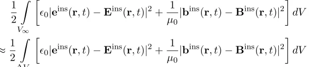
Combining Eq. (64) with Eq. (62), inserting the result into Eq. (61), then performing the volume integration on the left-hand side of Eq. (61) by using the fact that the macroscopic sources and fields are nearly uniform over the electrically small macroscopic volume ΔV, one obtains
∂P
∂t ·E− ∂B
∂t ·M≈
1 ΔV
ΔV
j·edV + 1 2ΔV
d dt
ΔV
0|eins−Eins|2+ 1
μ0|
bins−Bins|2
dV . (66)
Integration of this last equation from time t0 to time tgives
t
t0
∂P(r, t)
∂t ·E(r, t
)− ∂B(r, t)
∂t ·M(r, t )dt
≈ 1
ΔV t
t0
ΔV
j·edV dt+ 1 2ΔV
ΔV
0|eins−Eins|2+ 1
μ0
|bins−Bins|2 t
t0 dV
= 1
ΔV t
t0
ΔV
j·edV dt (67)
+ 1
2ΔV
ΔV
0|eins(r, t)−Eins(r, t)|2+ 1
μ0|
bins(r, t)−Bins(r, t)|2−0|eins(r, t0)|2− 1
μ0|
bins(r, t0)|2
dV
becauseEins(r, t0) = 0 andBins(r, t0) = 0.
This result shows that the change in macroscopic polarization energy in ΔV determined by the left-hand side of Eq. (67) is not just equal to the work done by the microscopic electric field on the microscopic current density (the mechanical energy represented by the double integral on the right-hand side of Eq. (67)) because of the additional change in field energy on the right-hand sides of Eq. (67). We will show next that this additional field energy produced by the dipoles inside any one macroscopic volume ΔV is confined to that ΔV and thus behaves as an isolated capacitive and inductive energy of the system of dipoles inside ΔV.