Shortest Path Analysis Based on Dijkstra’s Algorithm in Myanmar Road Network

Shortest Path Analysis Based on Dijkstra’s Algorithm in

Myanmar Road Network

Yi Yi Win

_{, Hnin Su Hlaing}

_{, Tin Tin Thein}

1, 2

_{Faculty of Computer Science, University of Computer Studies, Loikaw, Myanmar}

yiyipku941@gmail.com, hninsuhlaing07@gmail.com, tintinthein@ucspkku.edu.mm

Abstract:

The shortest path problem based on the data structure has become one of the hot research topics in graph theory. In modern life, everyone needs to reach their destinations in time. Distance calculator helps the system to find the distance between cities and calculate by traffic in both mile and time. The aim of this study is to provide finding the shortest path for bus routing based on Dijkstra’s algorithm (DA). As the basic theory of solving this problem, DA has been widely used in engineering calculations. DA is used to find the shortest path from one node to another node in a graph. DA is also known as a single source shortest path algorithm. This system acquired data from the geographic information system (GIS) of Cities in Myanmar.

Keywords: Directed Graph, Dijkstra’s Algorithm, GIS

1.

Introduction

Generally, in order to represent the shortest path problem we use graphs. A graph is a mathematical abstract object, which contains sets of vertices and edges. Edges connect pairs of vertices. Along the edges of a graph it is possible to walk by moving from one vertex to other vertices. In the real world it is possible to apply the graph theory to different types of scenarios. For example, in order to represent a map we can use a graph, Cities of Country in Myanmar where vertices represent cities and edges represent routes that connect the cities. Due to the different purposes the travel of the passengers and its transport requirements are different. For example, for business travel, the passenger wants the time of travel as short as possible. Tourists prefer the cost of travel as minimum as possible. There exist different types of algorithms that solve the shortest path problem. However, only several of the most popular conventional shortest path algorithms along with one that uses Dijkstra’s algorithm are

going to be discussed in this paper, and they are Dijkstra’s Algorithm, Floyd-Warshall Algorithm and Bellman-Ford Algorithm.

Sommer (2010) investigated shortest path query processing in networks both from a theoretical and a practical point of view. An experimental study was performed using road transportation network. The study revealed a simple and general method based on Voronoi duals to efficiently support the shortest path queries in undirected graphs with very low pre-processing overheads and competitive query times, at the cost of exactness. This method was proved to be effective on a variety of graph types while remaining a reasonable alternative toexisting exact methods specifically designed for transportation networks [8, 9, 12].

Pallottino and Scutella (1997)reported on Shortest Path Algorithms in Transportation models: classical and innovative aspects. They reviewed theshortest path algorithms in transportationsin two parts. The first part includes classical primal and dual algorithms which are the most interesting in transportation, either as a result of theoretical considerations or as a result of their efficiencies, and in view of their practical use in transportation models. They discussed the Promising re-optimization approaches involved. The second part includes dynamic shortest path problems that arise frequently in the transportation field. They analyzed the main features of the problems present under suitable conditions on travel time and cost functions, a general “chronological” algorithmic paradigm,called Chrono-SPT[7].

Dijkstra (1959) proposed a graph search algorithm that can be used to solve the single-source shortest path problem for any graph that has a non-negative edge path cost. This graph search algorithm was later modified by Lee in 2006 and was applied to the vehicle guidance system. This vehicle guidance system is divided into two paths; namely, the shortest path and the fastest path algorithms (Chen et al., 2009). While the shortest path algorithm focuses on route length parameter and calculates the shortest route between each OD pair, the fastest path algorithm focuses on the path with minimum travel time. The future travel time can be predicted based on prediction models using historical data for link travel time information which can be daily, weekly or even a session [2, 4, 11].

The aim of this paper is to apply Dijkstra algorithm for finding shortest path in the Cities of Myanmar. Data are acquired from geographic information system (GIS) which are used for searching routing architecture from Mandalay to Naypyitaw. The rest of this paper is organized as follows. The related methodologies are described in section2 and analyzing the experimental results are described in section 3.

2.

Methodologies

2.1.The Shortest Path algorithm

The objective is to find the shortest path of a given city, called home, toanother given city called destination. The length of a path is assumed to be equal to the sum of the lengths of links between consecutive cities on the path. With no loss of generality we assume that city 1 is the home city and city n is the destination. So, the basic task is: find the shortest path from city 1 to city n. For the technical reasons, and with no loss of generality, it is convenient to assume that city 1 does not have any immediate predecessor.

This is a mere formality because if this condition is not satisfied. And in view of our interest in DA, we shall focus on the shortest path problems where there might be cycling but the inter-city distances are non-negative. Different types of the shortest path algorithm are used to determine the shortest path of a graph. The most frequently encountered path is the shortest path of two specified vertices, the shortest path to all pairs of vertices, and the shortest path from a specified vertex to all others. The Dijkstra’s algorithm is the most efficient algorithm used to find the shortest

path of a known vertex to other vertices. Some improvements on Dijkstra’s algorithm are done in terms of efficient implementation.

2.2. Shortest path analysis based on

Dijkstra’s algorithm

The problem of finding the shortest path from a specified vertex s to mother t can be stated as follows: A simple weighted digraph G of n vertices is described by an n by n matrix D = [dij], where dij = length (or distance or weight) of the directed edge from vertex i to vertex j: Dijkstra’s algorithm labels the vertices of the given digraph, at each stage in the algorithm some vertices have permanent labels and others temporary labels. The algorithm begins by assigning a permanent label 0 to the starting vertex s, and temporary label infinity to the remaining n-1 vertices. Then, another vertex sets a permanent labelin each iteration, according to the following rules: [2, 4].

A. Every vertex j that is not yet permanently labelled gets a new temporary label whose value is given by min [old label of j, (old label of i + dij)], where i is the latest vertex permanently labelled, in the previous iteration, and dijis the direct distance between vertices i and j. if i and j are not joined by an edge, the dij = infinity. B. The smallest value of all the temporary

Dijkstra’s algorithm are of two types: temporary

and permanent. A temporary label is modified if a

shorter route to a node can be found. If no better route can be found, the status of the temporary label is changed to permanent.

Step 0: Label the source node (node 1) with the permanent label [0, --], set i =1.

Step i:

(a) Compute the temporary labels [ui + dij, i] for each node j that can be reached from node i, provided j is not permanently labelled. If node j is already labelled with [uj + k] through another node

k and if ui + dij <uj, replace [uj, k] with [ui + dij, i].

(b) If all the nodes have permanent labels, stop. Otherwise, select the label [ur, s] having the shortest distance (=ur) among all the temporary labels (break tie arbitrarily). Set i = r and repeat step i. [8, 9, 10]

This paper has proposed the optimization of algorithm based on the data structure, which has very important significance for improving the efficiency of solving the shortest path algorithm. This paper has proposed an optimization method which has mainly improved the nodes selection of the shortest path and data storage structure and

organization. Through comparison and analysis, the improved algorithm has been obtained, which has reduced the storage space and improved the operational efficiency.

3.

Results and Discussion

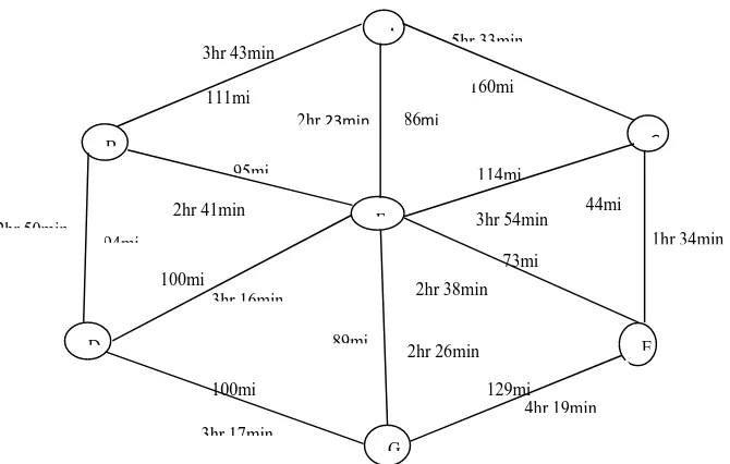
The effectiveness of the application area is governed Cities of Country in Myanmar. In this study, we propose a conventional measurement method of moored ship motions by using GPS position data. In Myanmar have many cities. From these cities, the system was display to take shortest distance from Mandalay to Naypyitaw as a destination and provide services between it and other cities and towns across Mynmar. In this paper, we not only use Dijkstra algorithm to implement the National City traffic advisory procedures which can satisfy the passengers’ different demand of travel and provide some optimal decision. The following table 2 shows the names of location and nodes identification.

Table 2. Nodes identification for Cites in Myanmar

This system will show the application area is about Cities of Country in Myanmar by using GPS position data. Permissible Route of the Road from Mandalay through Naypyitaw

LOCATION NODES

Mandalay A

Bagan B

Taunggyi C

Magway D

Kalaw E

Meiktila F

Fig 1. Permissible Route of the Road from Mandalay through Naypyitaw.

3.1. Calculation of Dijkstra’s

algorithm for Myanmar’s Cities

Edsger Dijkstra invented an algorithm for finding the shortest path through city to another. The following is a simple set of instructions that enables to follow the algorithm:

Step 1Label the start vertex as 0.

Step 2Box this number (permanent label).

Step 3 Label each vertex that is connected to the start vertex with its distance (temporary label).

Step 4Box the smallest number.

Step 5 From this vertex, consider the distance to each connected vertex.

Step 6If a distance is less than a distance already at this vertex, cross out this distance and write in the new distance. If there was no distance at the vertex, write down the new distance. Step 7 Repeat from step 4 until the destination vertex is boxed.

Using Time & Path

Table 3. Impact of Distance & Time on Path

DISTANCE TIME SHORTEST_PATH

Min. Less Selected

Max. More Not Selected

Min. More Not Selected

Using Position & Path

Table 4. Impact of Distance & Position on Path

DISTANCE POSITION SHORTEST_PATH

Min. Accurate Selected

Max. Not Accurate Not Selected

3.2. Analytical Solution to the Problem

Table 2 and Table 3 are shows impact of distance on path and position on route. In shortest path algorithm, 129mi

3hr 43min

111mi

100mi

86mi

160mi

44mi

73mi

100mi 94mi

95mi 114mi

89mi

1hr 34min 2hr 50min

3hr 17min

2hr 23min

5hr 33min A

E

G

B C

D

F

3hr 16min

4hr 19min 2hr 26min

demand of travel and provides some optimal decision.

Step 1: Label A as 0 Step2: Box this number

Step3: Label value of 111mi (3hr 43min) at B, 160 mi (5hr 33min) at C And 86 mi (2hr 23min) at F.

Above the figures produce when the iteration of step 1, 2 and 3. This is show by travel traffic shortest path from Mandalay to Bagan, Meiktila and Taunggyi. The minimum distance selected at Meiktila.

Step 4: Box the 86 mi (2hr 23min) at F.

Step 5: From F, the connected vertices are B, C, D, E and G. The distance at these vertices are 181 mi (5hr 4min) at B (86+95)mi (2hr 23min +2hr 41min), 200mi(6hr 17min) at C (86+114)mi (2hr 23min +3hr 54min), 186mi (5hr 39min) at D(86+100) mi (2hr 23min +3hr 16min), 159mi (5hr 1min)at E(86+73)mi (2hr 23min + 2hr 38min) and 175mi (4hr 49min) at G (86+89) mi (2hr 23min +2hr 26min).

The following figure is show from step 4 and 5 achieve. From the minimum value to connected cities. As the distance at Bagan is 111mi (3hr 43min), lower than the 181mi (5hr 4min) currently, cross out the 181mi (5hr 4min), at Taunggyi is 160mi (5hr 33min) lower than the 200mi (6hr 17min), at Magway is 186mi (5hr 39min), at Kalaw is 159mi (5hr 1min) and at Naypyitaw is 175mi (4hr 49min).

Step 6: As the distance at B is 111mi (3hr 43min), lower than the 181mi (5hr 4min) currently at B, cross out the 181mi (5hr 4min), at C is 160mi (5hr 33min) lower than the 200mi (6hr 17min), at D is 186mi (5hr 39min), at E is 159mi (5hr 1min) and at G is 175mi (4hr 49min).

Step 4: Box the smallest number, which is the 111mi (3hr 43min) at B.

Step 5: From B, the connected vertices is D. The distance at these vertices is 205mi (6hr 33min) at D (111+94) mi (3hr 43min + 2hr 50min).

A

B C

F 0

111

160

86

A

B C

F 0

111 160

86

A

B

F

C

D

E

G 0

111

181

86

160

200

159

At the figure, box the smallest number, which is the 111mi (3hr 43min) at Bagan. From Bagan to connected Magway. As the distance at Magway is 186mi (5hr 39min), lower than the 205mi (6hr 33min) currently, cross out the 205mi.

Step 6: As the distance at D is 186mi (5hr 39min), lower than the 205mi (6hr 33min) currently at D, cross out the 205mi.

Step 4: Box the smallest number, which is the 159mi (5hr 1min) at E.

Step 5: From E, the connected vertices are C and G. The distance at these vertices are 203mi (6hr 35min) at C (159+44) (5hr 1min + 1hr 34min) and 288mi (9hr 20min) at G (159+129)mi (5hr 1min + 4hr 19min).

These figure, box the smallest number, which is the 159mi (5hr 1min) at Kalaw. From Kalaw, the connected are Taunggyi and Naypyitaw. The distance are 203mi (6hr 35min) and 288mi (9hr 20min).

159 205

A

B

F

C

D E

G 0

111

181 ₈₆

160

200

175 186

288

203

205

A

B

F

C

D

E

G 0

111

181 86

160

200

159

As the distance at Taunggyi is 160mi (5hr 33min), lower than the 203mi (6hr 35min) currently, cross out the 203mi and the distance at Naypyitaw is 175mi (4hr 49min), lower than the 288mi (9hr 20min) currently, cross out the 288mi.

Step 6: As the distance at C is 160mi (5hr 33min), lower than the 203mi (6hr 35min) currently at C, cross out the 203mi and the distance at G is 175mi (4hr 49min), lower than the 288mi (9hr 20min) currently at G, cross out the 288mi.

Step 7: The final vertex, in this case G, is not boxed. The boxed number at G is the shortest distance. The route corresponding to this distance of 175mi (4hr 49min) AFG, but this is not immediately obvious from the network.

The final result shows in minimum number at Naypyitaw. It is the shortest distance number. The route corresponding to this distance of 175mi (4hr 49min) from Mandalay to Meiktila to Naypyitaw.

3.3. Evaluation result of proposed system

This section described the evaluation result of proposed system which are compared in miles and hours. The following figure 2 shows the comparison results of shortest path analysis based on DA algorithm. That graph compared miles different from one city to another city through Mandalay to Naypyitaw. In this graph, Mandalay-Meiktila-Naypyitaw road is the shortest route compared with others routes. This results indicated that A-F-G have shortest distance (miles) rather than others.

. Fig.2 the distance different between cities through the goal city by mile

Figure 3 describes the comparison results of shortest path which is based of time spend calculation. According to this result A-F-G’s hours were consumed in passing the shortest distance.

0 50 100 150 200 250 300 350 400

A-B-F-G A-C-F-G A-C-E-G A-F-G A-B-D-G

M

il

es

City

0 2 4 6 8 10 12 14

A-B-F-G A-C-F-G A-C-E-G A-F-G A-B-D-G

H

o

u

rs

a

n

d

M

in

u

te

s

Fig.3 the distance different between cities through the goal city by hour/minute

4.

Conclusion

This paper discussed the shortest path analysis based on Dijkstra’s algorithm and implemented a routing system based on GIS which can be widely used in all sorts of services. Experiment results indicate that the proposed algorithm can not only solve the shortest path problem of undirected-graph but also can solve the shortest path problem of directed-graph. Finding shortest path is noat a solution all the time because there are several factors affecting travel time. Not only theoretical concept is given but also practical implementation is also given in this paper. This system revealed that evaluation result provides the optimal route from Mandalay through Naypyitaw. Further research is focused on integrating the DA algorithm with other A*,Floyd-Warshals algorithm & Bellman Ford algorithm etc.

5.

Reference

[1] Denardo, E.V. and Fox, B.L. (1979) Shortest-route methods: 1. Reaching, pruning, and buckets. Operations Research 27, 161–186.

[2] Dijkstra, E.W. (1959) A Note on Two Problems in Connexion with Graphs. Numerische Mathematik 1, 269–271.

[3] Feng, L. U. (2001). Shortest Path Algorithms: Taxonomy and Advance in Research [J]. Acta Geodaetica Et Cartographic Sinica, 3, 020.

[4] Goldberg, A. V. (n.d.). Point - to - Point Shortest Path Algorithms withPre-processing. Silicon Valley:MicrosoftResearch.

[5] J. Chamero, ―Dijkstra’s Algorithm‖ Discrete Structures & Algorithms, 2006.

[6] Liu Ping, An algorithm of shortest paths based on dijkstra algorithm, Journal of Value Engineering, 2008.1.

[7] Microsoft Shortest Path Algorithms Project:

research.microsoft.com/research/sv/SPA/ex.html. [8] Nar, D. (1997). Graph theory with applications to engineering and computer science. Prenctice Hall.

[9] Sommer, C. (2010). Approximate Shortest Path and Distance Queries in Networks. Tokyo: Department of Computer Science, Graduate School of Information Science and Technology. [10] T. Li, Q. a. (2008). An efficient Algorithm for the single source Shortest Path Problem in Graph Theory. International Conference on Intelligent System and Knowledge Engineering, (pp. 152 - 157).

[11] Zhang Yi, Application of Improved Dijkstra Algorithm in Multicast Routing Problem, Journal of Computer Science, 2009.8.