17
Shortest Path Algorithm using Hashing and Queue
Shruti Pant
M.Tech CSE
Uttarakhand Technical university Dehradun, India
Pooja khulbe
M.Tech CSE
Uttarakhand Technical university Dehradun, India
ABSTRACT
Finding the shortest path in a graph means selecting the path between source and destination which gives the minimum path length. This problem of finding the shortest path can be solved using Dijkstra algorithm. The time complexity of Dijkstra algorithm is high. Looking at the shortcoming of traditional Dijkstra algorithm, this paper has proposed a new method to improve the time complexity of this algorithm using queue and hashing techniques. The time complexity of the improved algorithm is O(n log n).
Keywords
Shortest path, Dijkstra algorithm, Queue, Hashing, Stack.
1. INTRODUCTION
The shortest path algorithm has gradually become one of the recent topics of research. It is used in geographic information science, operations research, computer science and other discipline. It is not only the key problem in network analysis but also the key issues in graph theory, electronics, network optimization, logistics and transportations. Shortest path means selecting the path from source to destination in which the path length is the minimum. This shortest path problem can be solved by Dijkstra algorithm. This algorithm is used to find the shortest path between any nodes. It solves the single source shortest path problem for a graph with non-negative edge path costs, producing a shortest path tree. The basic idea of Dijkstra algorithm is to find the shortest path between node N1 to node N2 i.e. for a given source vertex in the graph, the algorithm finds the path with lowest cost between that vertex and every other vertex. Then using this shortest path, find the shortest path between node N2 to node N3. Hence a shortest path is founded between node N1 to node N3. This process is repeated from source until the destination is reached. This idea of Dijkstra algorithm has the time complexity as O(n2). This paper has proposed the improved time complexity as O(n log n).
2. DIJKSTRA ALGORITHM
2.1 Description of traditional Dijkstra
Algorithm
Dijkstra algorithm can label the nodes constantly. The value of the label varies with the nodes, which is the length of the shortest path between the starting point and label nodes [3]. In addition, the nodeswithout labels can be labeled temporarily that is, the relative minimum value of the shortest distance for the other nodes is given. Of course, the closer the starting point approaches the vertex, the earlier it gets the fixed label. Combining with the backtracking algorithm we can find the node passed by the shortest path between the starting point and the other nodes, and then obtain the shortest path labeled by the node [4].
2.2 Shortcomings of Dijkstra’s Algorithm
The Dijkstra algorithm takes a large amount of time in calculating the shortest path. So it is not applicable when the number of nodes increases. As the shortest path finds an application in networking, transportation, etc so there is a need to find the shortest path in lesser time. It also takes lots of space for cost matrix due to which space complexity increases.3. NEW IMPROVED DIJKSTRA
ALGORITHM
3.
3.1 Proposed Algorithm
Step1- Enter the adjacency list ADJ which contains the node number and the edge weight.
Step2- Arrange each row of adjacency list in ascending order of edge weight using shell sort.
Step3- Enter the source and destination.
Step4- Mark the status of each node as NULL in STATUS. Step5- Mark the weight of each node as infinity and source weight as zero in LIST.
Step6- insert source in QUEUE.
Step7- Repeat steps till QUEUE is not empty.
a) Delete element X from FRONT end of QUEUE. b) if STATUS[X]=NULL then-
i. If neighbor of X is not present in QUEUE then add X’s neighbor to QUEUE.
ii. Calculate the weight of its neighbors as- iii. Min(Wij, eij+ parent’s weight).
iv. If the new weight is less than the weight present before then insert this calculated weight in LIST and update its parent in LIST.
v. Update STATUS[X]=X. Else
Delete the element from the QUEUE. Step8- set y = destination.
18
3.1.1 Working of algorithm
First enter the adjacency list. Arrange each row of the adjacency list in ascending order using shell sort according to edge weight entered so that there is a right selection of nodes for finding the path. STATUS is a single dimensional array used for keeping track that if the node has already been visited or not. For this STATUS of each node is set as NULL, when the node is visited then its status is updated with the node number. If the STATUS of node number is NULL means that the node has not been visited but if it’s NOT NULL then the node is visited. LIST is a two dimensional array of structure containing the weight of the node and parent of the node. Firstly the weight of each node in LIST is marked as infinity, after calculating the weight through parent node the weight of node is updated when visited. Queue is used for updating the weight of each node by selecting the neighbor nodes according to the adjacency list. By this all the node’s weight is calculated. Each time a node is deleted from front of the queue and its neighbors are added to the queue. If the neighbor already exists then just its weight is calculated like other neighbor’s weight. If the calculated weight is less than the existing weight of the neighbor then its weight is updated in LIST. This loop continues till queue is not empty. Stack is used for finding the path between source and destination by setting a variable equal to the destination and recursively visiting its parent so that the path can be found. This loop continues till source is not reached.
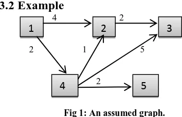
3.2 Example
4 2
2 1 5
[image:2.595.318.548.108.228.2]2
Fig 1: An assumed graph.
Step 1- Adjacency matrix ADJ.
Table1: Adjacency matrix entered by user.
Step 2- Sort this list according to edge weights using shell short.
Table 2: Adjacency matrix after shell sort.
Step 3- Source=1 and destination=3. Step 4- Initialize status.
1 2 3 4 5
NULL NULL NULL NULL NULL
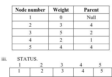
Step 5- Initialize LIST.
Table 3: LIST which stores the weight and parent of each node.
Node
number Weight Parent
1 0 Null
2 Infinite
3 Infinite
4 Infinite
5 Infinite
Step 6- QUEUE.
1 2 3 4 5 1
Step 7- Delete X i.e. X= 1.
i. Add neighbor of 1 to QUEUE.
1 2 3 4 5 4 2
[image:2.595.55.232.372.486.2]ii. Calculate the weight of added nodes and add the minimum weight of each added node to LIST. Table 4: Updated LIST after accessing the first node.
Node
number Weight Parent
1 0 Null
2 4 1
3 Infinite
4 2 1
5 Infinite Nod
e no.
Adjacent node 1
Adjacent node 2
Adjacent node 3 Node
no.
Edge wt
Node no.
Edge wt
Node no.
Edge wt
1 2 4 4 2
2 3 2
3 NULL
4 5 2 2 1 3 5
5 NULL
Node no.
Adjacent node 1
Adjacent node 2
Adjacent node 3 Node
no.
Edge wt
Node no.
Edge wt
Node no.
Edge wt
1 4 2 2 4
2 3 2
3 NULL
4 2 1 5 2 3 5
5 NULL
1
2
3
[image:2.595.347.515.652.744.2]19 iii. STATUS.
1 2 3 4 5 1 NULL NULL NULL NULL
Step 8- Delete X i.e. X=4 from QUEUE. i. Add neighbor of 4 to QUEUE.
1 2 3 4 5 2 5 3
ii. Calculate the weight of added nodes and add the minimum weight of each added node to LIST. Table 5: Updated LIST after accessing second node.
Node number Weight Parent
1 0 Null
2 3 4
3 7 4
4 2 1
5 4 4
iii. STATUS.
1 2 3 4 5 1 NULL NULL 4 NULL
Step 9- Delete X i.e. X=2 from queue.
i. Add neighbor of 2 to QUEUE. As neighbor of 2 i.e 3 already exist in the QUEUE, so just its weight is calculated by using 2 as parent.
1 2 3 4 5 5 3
ii. Calculate the weight of added nodes and add the minimum weight of each added node to LIST. Table 5: Updated LIST after accessing third node.
Node number Weight Parent
1 0 Null
2 3 4
3 5 2
4 2 1
5 4 4
iii. STATUS.
1 2 3 4 5 1 2 NULL 4 NULL
Step 10- Delete X i.e. X=5.
i. It has no neighbors, so QUEUE remains the same. 1 2 3 4 5
3
ii. Calculate the weight of added nodes and add the minimum weight of each added node to LIST. Table 6: Updated LIST after accessing fourth node.
Node number Weight Parent
1 0 Null
2 3 4
3 5 2
4 2 1
5 4 4
iii. STATUS.
1 2 3 4 5 1 2 NULL 4 5
Step 11- Delete X, i.e. X=3.
i. It has no neighbors, so QUEUE remains the same. Now QUEUE has become empty so it will come out of loop.
1 2 3 4 5
ii. Calculate the weight of added nodes and add the minimum weight of each added node to LIST. Table 7: Updated LIST after accessing fifth node.
Node number Weight Parent
1 0 Null
2 3 4
3 5 2
4 2 1
5 4 4
iii. STATUS.
1 2 3 4 5 1 2 3 4 5
Step 12- Destination i.e. y=3 (this loop continues till source is not reached).
[image:3.595.322.519.444.580.2]i. Stack- push y in stack.
Fig 2: Stack after pushing destination. 3
20 ii. Push parent of 3 (select parent from LIST).
Fig 3: Stack after pushing parent of 1st node.
iii. Push parent of 2 (select parent from LIST).
Fig 4: Stack after pushing parent of 2nd node.
iv. Parent of 4 is 1 i.e source is reached so it will come out of loop. For printing the shortest path first print the source and then one by one stack elements from the top till stack is not empty.
3.3 Analysis of new algorithm
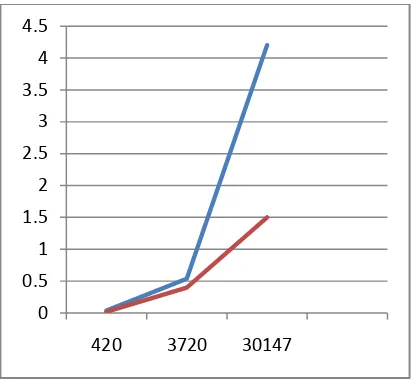
[image:4.595.316.523.70.261.2]The new algorithm has improved the time complexity. The time complexity of traditional Dijkstra algorithm is O(n2) while the time complexity of this new algorithm is O(n log n). It can be seen form the following table that this algorithm is improved the working of traditional Dijkstra algorithm-
Table 8: Comparison between traditional Dijkstra algorithm and new improved algorithm.
Original Data Traditional
Dijkstra Algorithm
Improved Dijkstra Algorithm
Arc Node Total
No. of paths
Com putin g Time (s)
Total No. of path
Computi ng time (s)
420 132 387 0.04 87 0.02
3740 1475 4213 0.54 139 0.4 30147 11655 84531 4.2 844 1.5
Fig 4: Comparative study of the two algorithms.
This graph depicts the comparative study of the Dijkstra algorithm and the new proposed algorithm. In this blue line represents Dijkstra algorithm and red line represents New proposed algorithm.
4. CONCLUSION
Dijkstra algorithm is used in various fields. This paper has found the application of Dijkstra algorithm in those fields. By using queue, stack and hashing it has improved the running time of the algorithm which was earlier very large. By this the need to find the shortest path in less time can be solved easily.
5. FUTURE SCOPE
This algorithm has used linear data structure and has improved the time complexity of traditional Dijkstra algorithm. Linear data structure is easy to implement. In the similar way traditional Dijkstra was improved using min heap. In future this algorithm can further be improved by improving its space complexity as well as it time complexity as linear time.
6. REFERENCES
[1] Y.Cao, “The Shortest path algorithm in data structures”, Yibin University, vol. 6, 2007, pp.82-84.
[2] Q. Sun, J. H. Shen, J. Z Gu, “An improved Dijkstra algorithm”, Computer Engineering And
Applications, vol. 3, 2002, pp. 99-101.
[3] Jinhao Lu, Chi Dong, Research of the shortest path algorithm based on the data structure [J], IEEE, 2012, pp. 108-12.
[4] L.B. Chen, R.T Liu, “A dijkstra’s shortest path algorithm”, Harbin University of Technology, vol 3, 2008,pp.35-37.
[5] F.S.XU,C.Tian, “All the Shortest Path Algorithm”, Computer Engineering and Science, vol.12, 2006, pp.83-84.
[6] Y. Tang, Y. Zhang, H. Chen, “A Parallel Shortest Path Algorithm Based on Graph-Partitioning and Iterative Correcting”, in Proc. of IEEE HPCC, pp. 155-161, 2008.
0 0.5 1 1.5 2 2.5 3 3.5 4 4.5
420 3720 30147
2 3
4 2 3
TOP
[image:4.595.51.267.481.600.2]21 [7] Fuhao ZHANG, Ageng QIU, Qingyuan LI,”
Improve on dijkstra shortest path algorithm for huge data”, ISPRS, 2009.
[8] Noto m, Sato h.,” Improved Dijkstra algorithm for network routing” Systems, man and cybermatics, IEEE international conference, vol 3, pp 2316 – 2320, 2000.
[9] Yizhen Huang, Qingming Yi, Min Shi, “An Improved Dijkstra Shortest Path Algorithm”, Proceedings of the 2nd International Conference on Computer Science and Electronics Engineering (ICCSEE 2013), pp. 0226-0229, 2013.
[10]
F.S. XU. “Shortest path calculation algorithm”.Computer Applications, vol 5, pp.88-89, 2004.