Comparison of fuzzy and crisp classification trees using gini index, chi-square statistic and the gain ratio

COMPARISON OF FUZZY AND CRISP CLASSIFICATION TREES USING

GINI INDEX, CHI-SQUARE STATISTIC AND THE GAIN RATIO

MUCHAI, EUNICE WAMBUI

REG.NO. I84/13318/2009

A THESIS SUBMITTED IN FULFILMENT OF THE REQUIREMENTS FOR THE AWARD OF DEGREE OF DOCTOR OF PHILOSOPHY (STATISTICS) IN THE SCHOOL OF PURE

AND APPLIED SCIENCES OF KENYATTA UNIVERSITY

ii

DECLARATION

This thesis is my original work and has not been presented for any other degree or award in any university

Muchai, Eunice Wambui

Signature ………. Date………

This thesis has been submitted with our approval as university supervisors.

Prof. L. O. Odongo

Signature ………. Date………

Department of Statistics and Actuarial Science

Kenyatta University

Dr. J. K. Kahiri

Signature ………. Date………

Department of Statistics and Actuarial Science

iii

DEDICATION

iv

ACKNOWLEDGEMENT

I am most grateful to God for His Mercy and Grace extended to me through the years and in particular, during the period of this study.

To Prof. L.O., Odongo thank you for your unwavering patience, availability and invaluable guidance throughout the study. To Dr. J.K., Kahiri your timely comments and guidance made the completion of this work possible.

I really appreciate my husband and children who encouraged me when I almost gave up.

I wish to thank the entire staff of Statistics and Actuarial Science, Department of Kenyatta University for encouraging me.

v

TABLE OF CONTENT

DECLARATION ... ii

DEDICATION ...iii

ACKNOWLEDGEMENT ... iv

TABLE OF CONTENT ... v

LIST OF TABLES ... vii

ABSTRACT ... viii

CHAPTER ONE... 1

INTRODUCTION ... 1

1.1 Background Information ... 1

1.2 Classical classification ... 2

1.2.1 Linear Discriminant Rule ... 3

1.2.2 Bayes’ Discriminant Rule ... 3

1.3 Classification trees ... 5

1.3.1 Fuzzy classification trees ... 8

1.4 Statement of the problem ... 12

1.5 Justification ... 13

1.6 Objectives ... 13

1.6.2 Specific Objectives ... 13

1.7 Significance of the study ... 14

1.8 Outline of the thesis ... 14

CHAPTER TWO ... 15

LITERATURE REVIEW ... 15

2.1 Introduction ... 15

2.2 Classical classification ... 15

2.3 Crisp Classification trees ... 16

2.4 Fuzzy classification trees ... 17

CHAPTER THREE ... 19

METHODOLOGY ... 19

3.1 Introduction ... 19

3.2 Classification Trees ... 19

vi

3.2.2 Assigning Classes to Tree Nodes ... 20

3.3 Impurity Measures ... 20

3.3.1 The Gini Index ... 22

3.3.2 Pearson’s chi –squared statistic ... 24

3.3.3 Gain ratio ... 32

3.4 Testing for Differences in Performance among the Trees... 36

CHAPTER FOUR ... 38

COMPARISON OF CRISP AND FUZZY CLASSIFICATION USING DIFFERENT IMPURITY MEASURES ... 38

4.1 Introduction ... 38

4.2 Results from 3-variate normal populations based on simulated data ... 38

4.2.1 Testing for difference in performance of the impurity measures for simulated data ... 42

4.2.2 Different Sample Sizes of population one and population two from the 3-variate normal populations simulated data ... 43

4.3 Results from 3-variate normal populations based on real data ... 46

4.4 Results from 4-variate normal populations based on simulated data ... 52

4.4.1 Conclusion from simulated data ... 54

4.5 Results from 4-variate normal populations based on real data ... 55

4.5.1 Splitting Variables Results... 57

4.5.2 Conclusion from real data ... 65

CHAPTER FIVE ... 66

SUMMARY, CONCLUSION AND RECOMMEDATIONS ... 66

5.1 Introduction ... 66

5.2 Summary ... 66

5.3 Conclusion... 66

5.4 Recommendations ... 68

REFERENCES ... 69

APPENDIX I ... 72

IRIS DATA SET ... 72

APPENDIX II ... 75

vii

LIST OF TABLES

Table 4.1: Probabilities of Correct Allocation for Gini Index, Pearson’s Chi-squared Statistic and

Gain Ratio ... 40

Table 4.2: Proportion of times crisp probabilities outperforms fuzzy probabilities ... 41

Table 4.3:McNemars Values for Gini Index, Pearson’s Chi-squared statistics and Gain Ratio ... 42

Table 4.4a: Probability of correct allocation to population one for different sample sizes ... 44

Table 4.4b: Probability of correct allocation to population two for different sample sizes ... 45

Table4.5: Instances Individuals Are Allocated to Right and Left Branches ... 49

Table 4.6a: Information Gain calculated Values ... 50

Table 4.6b: Intrinsic information calculated values ... 50

Table 4.6c: Gini Index, Pearson’s Chi-Squared and Gain Ratio calculated values ... 50

Table 4.7: Probabilities of correct allocation ... 51

Table 4.8: McNemars values for real data... 52

Table 4.9: Probabilities of Correct Allocation using simulated data ... 53

Table 4.10: McNemar’s values for simulated data ... 54

Table 4.11: Proportion of times crisp probabilities outperforms fuzzy probabilities ... 55

Table 4.12: Allocation of individuals using Sepal length ... 57

Table 4.13: Allocation of individuals using Sepal width ... 58

Table 4.14: Allocation of individuals using Petal length ... 59

Table 4.15: Allocation of individuals using Petal width ... 60

Table 4.16:Gini Index, Pearson’s chi-squared and Gain ratio values at different points ... 61

viii

Table 4.18: Gini Index, Pearson’s chi-squared and Gain ratio values ... 64 Table 4.19: Probabilities of allocation for the iris data ... 65

ABSTRACT

1

CHAPTER ONE

INTRODUCTION

Classification is a branch of Statistics that identifies which of a set of categories or classes, a new individual belongs. This is done on the basis of measurements on one or more of the attributes (variables)

of an individual. A criterion or classification rule is applied on the individual’s measurements to

determine which category (class) the individual observation belongs. Since this applies probability theory,

it is possible that an individual maybe allocated to the wrong class. The probability of allocating an

individual to the wrong class is known as probability of misclassification. A good classification rule

minimizes the probabilities of misclassification.

2

have used classification techniques to predict whether a company will go bankrupt or not (Altman, 1968). Discriminant analysis has also been applied to a war data set, where a discriminant model was used to predict who would win a battle given some characteristics from the Second World War (Chalikias et al., 2009). Classification has also been applied in artificial intelligence, especially in pattern recognition (Hastie et al., 1995).

Many different models of classification are in use today. In all the models, the guiding principle is to minimize the probabilities of misclassification. Classification should also be done within acceptable time and with reasonable effort. Below is a brief description of some classification models in use.

1.2Classical classification

Consider g mutually exclusive and exhaustive populations denoted by ₁,₂,..,._g where g ≥2. Assume that each individual in population _ican be described by a p-dimensional random

vector 







 X X Xp

X ₁, ₂,..., with corresponding density function given by fi(x,) i=1, 2,. . . , g,

defined on p-dimensional real space p

. Let the corresponding mean vector and dispersion matrix be given by µi and Σi respectively.

Then classification (or discrimination) procedures involve partitioning the sample space p into

g disjoint subsets R1, R2, . . ., Rg such that

1

g p

i i

R



  , and then allocating an individual

observation X to _i if XR_i



3 1.2.1 Linear Discriminant Rule

A rule d which allocates X to ∏i if XRi is called a discriminant rule. The classical linear

discrimnant rule allocates X to ∏j if it maximizes



 



1 _{ }

 

_  _

That is, allocate an individual with characteristic X to ∏j if;



  



 



i j

j x x x

x 1  max  1  i, j =1, 2,…, g (1.1)

Under multivariate normal assumption this is equivalent to maximizing the likelihood function. That is allocate X to

 

 

if _i

i j

j max

 i, j = 1, 2, . . . , g (1.2)

Where Li denotes the likelihood function of X.

1.2.2 Bayes’ Discriminant Rule

The Bayes’ discriminant rule allocates a new observation X to j if;

 

 

L _{i i}

i j

j max , 1,2,...,

 (1.3)

Where _iis the prior probability of an observation belonging to population_i.

Suppose that the g populations are normally distributed. That is if X comes from the population ,

i

 then X is normally distributed with mean vector i

4

allocation rule will allocate a new observation X to _j if ;

 

 

L i i

i j

j max , 1,2,...,



That is, allocate x to _j if;

 



 



j  x  x 

 ₂ 1

1 2 2 1 exp 2 =

 









i x x

i

 



 ₂ 1

1 2 2 1 exp 2

max i, j=1, 2, …,g (1.4)

This implies that the Bayes’ allocation rule will allocate x to _j if;





 

j x  x 

 ₂ 1

1

2 1

exp ≥



 



     _{ } _{ }    i i i i

i x  x 

 1

2 1

2 1

exp i, j = 1,2, . ..g,

(1.5)

That is, allocate x to j if;



 





 







i j i j x x x

x    

                  1 1 2 1 2 1 2 1

exp i, j= 1, 2, . . . , g (1.6)

If g =2 then, in this case there are two populations ₁ and ₂and the Bayes’ rule will allocate

x to ₁ if;



 

 

 







1 2 ' 2 1 1 1 1 2 1 2 2 1 1 2 1 ' 2 1

exp    

                  x x x

5

Otherwise it will allocate x to ₂.

1.3Classification trees

6

Figure 1.1: Classification tree for credit customers

Altman, (1968)

7

The original data, known as the root node, was partitioned into two or more non-overlapping sub-samples (or children nodes). The partitioning is done based on one of the independent variables known as the splitting attribute(variable). Each instance in the root node is sent down one of the branches (depending on its value of the splitting attribute) into one of the nodes. The splitting attribute is the attribute that will partition the original sample into sub-samples that are as homogenous (or pure) as possible. If a variable has more than one value, the value that gives the most homogenous sub-samples is used.

The process is repeated for each of the subsequent nodes. By considering the cases in a particular node the node is partitioned and new nodes are created. This process is repeated for each node until some rule is violated. When this happens, the node is not partitioned further and such a node is referred to as leaf or terminal node. The whole process is terminated when there are only leaf nodes left. Each leaf node is assigned one class representing the most appropriate target value. (Maimon and Rokach, 2010).

Three issues are to be considered in classification trees. These are; how to select the splitting attribute, when to stop splitting and how nodes are assigned to classes.

The splitting attribute is selected by using an impurity measure and classes are assigned at the terminal nodes. These will be further discussed in chapter three.

8 1.3.1 Fuzzy classification trees

Fuzzy classification trees are a fusion of fuzzy sets and decision trees. The fundamental difference between fuzzy and crisp trees is that with fuzzy decision trees, gradual transitions exist between attribute values. For the crisp classification the tree allows for abrupt transition. Fuzzy classification trees are the more natural approach. The early approaches to using fuzzy models were to fuzzify the whole data set. This is quite cumbersome and for big data sets is time consuming. A more recent approach is to fuzzify the decision point only (Janikow1996). Below is an introduction of fuzzy theory.

1.3.1.1 Fuzzy sets and approximate reasoning

Fuzzy sets were introduced by Zadeh (1965) to represent and manipulate data and process information when there are uncertainties which are non statistical. It was specifically designed to mathematically represent vagueness and to provide formalized tools for dealing with the imprecision intrinsic to many problems. Fuzzy logic provides an inference morphology that enables approximate human reasoning capabilities to be applied to knowledge-based systems. The theory of fuzzy logic provides a mathematical strength to capture the uncertainties associated with human cognitive processes, such as thinking and reasoning (Zadeh, 1965).

In fuzzy logic, exact reasoning is viewed as a limiting case of approximate reasoning and everything is a matter of degree, where knowledge is interpreted as a collection of elastic or, equivalently, fuzzy constraint on a collection of variables. In fuzzy reasoning, inference is viewed as a process of propagation of elastic constraints hence any logical system can be fuzzified.

9

estimated values under incomplete or uncertain information. This gives fuzzy systems better performance for some applications.

In set theory, a subset A of a set X can be defined by a function χA as a mapping from the elements of X to the elements of the set {0, 1}, χA: X → {0, 1}.

This mapping is represented as a set of ordered pairs, with one ordered pair present for each element of X. The first element of the ordered pair is an element of the set X, and the second element is an element of the set {0, 1}. The value zero is used to represent complete non-membership, and the value one is used to represent complete membership. The truth or falsity of the statement, ”x is in A”, is determined by the ordered pair (x, χA(x)). The statement is true if the second element of the ordered pair is 1, and the statement is false if it is 0.

A fuzzy subset A of a set X can be defined as a set of ordered pairs, each with the first element from X, and the second element from the interval [0, 1], with exactly one ordered pair present for each element of X. This defines a mapping, μA, between elements of the set X and values in the interval [0, 1]. The value zero is used to represent complete non-membership, the value one is used to represent complete membership, and values in between are used to represent intermediate degrees of membership.

10

Definition 1.1 (Zadeh, 1965): Let X be a nonempty set. A fuzzy set A in X is characterized by its membership function μA, X → [0, 1] and μA(x) is interpreted as the degree of membership of element x in fuzzy set A for each xX

It is clear that A is completely determined by the set of tuples A = {(x, μA(x))|xX } Frequently one writes simply A(x) instead of μA(x). The family of all fuzzy subsets in X is denoted by F(X). Fuzzy subsets of the real line are called fuzzy quantities.

Let B be a fuzzy subset of X, the support of B, denoted supp(B), is the crisp subset of X whose elements all have nonzero membership values in B.

That is,





)

(B  xX B x  Supp

Let X be a classical set, then a fuzzy subset B of X is called normal if there exists anxX such that B(x) = 1. Otherwise B is said to be subnormal.

Definition 1.2(Zadeh, 1965): An α-level set of a fuzzy set A of X is a non-fuzzy set denoted by [A]α and is defined by,

 

  

  

 

0 ),

(

0 }, ) ( / {

   

A Supp cl

t A X t A

where cl (suppA) denotes the closure of the support of A.

11

examples of fuzzy numbers. Using the theory of fuzzy subsets we can represent these fuzzy numbers as fuzzy subsets of the set of real numbers. More exactly, a fuzzy number A is a fuzzy set of the real line with a normal, (fuzzy) convex and continuous membership function of bounded support. The family of fuzzy numbers is denoted by F.

Definition 1.3 A fuzzy set A is called triangular fuzzy number with peak (or center) a, left width α >0 and right width β >0 if its membership function has the following form

                    otherwise a t a a t a t a t a t A 0 , 1 , 1 ) (     (1.8)

and is denoted by A = (a, α, β). (Zadeh, 1965)

Definition 1.4 A fuzzy set A is called trapezoidal fuzzy number with tolerance interval [a, b], left width α and right width β if its membership function has the following form

12

A trapezoidal fuzzy number may be seen as a fuzzy quantity “x is approximately in the interval [a, b]”.(Francesco, 2010)

1.3.2 Crisp classification trees

This is a classification tree where the splitting value, x, is a crisp value. Suppose then a subset A of a set X can be defined by a function χA as a mapping from the elements of X to the elements of the set {0, 1}, χA: X → {0, 1}.

This mapping is represented as a set of ordered pairs, with one ordered pair present for each element of X. The first element of the ordered pair is an element of the set X, and the second element is an element of the set {0, 1}. The value zero is used to represent complete non-membership, and the value one is used to represent complete membership. The truth or falsity of the statement, ”x is in A”, is determined by the ordered pair (x, χA(x)). The statement is true if the second element of the ordered pair is 1, and the statement is false if it is 0.

1.4 Statement of the problem

Work on crisp classification trees has been introduced as a nonparametric discriminant method. (Yu-Shin, 2004; Dobra, 2002). With the introduction of fuzzy logic, researchers started using fuzzy classification trees, which have the ability to deal with numeric, missing or inaccurate data ( Dorokhov and Chernov,2011) . For example (Hashemi et al., 2008) applied fuzzy decision trees to classify data streams in the presence of noise. Zeinalkhani and Eftekhari (2011)

presented a criteria for stopping fuzzy trees. According to Dorokhov and Chernov (201 ) fuzzy decision tree allows one to consider the uncertainty of estimations of decisions. Fuzzy trees may also supposes the use of qualitative presentations. Since the fuzzy classification trees are applied in

13

comprised. This may be done by comparing their performance to that of crisp classification trees. In this work performance of fuzzy classification trees and crisp classification trees are compared. This is done using Gini index, Pearson’s Chi-squared statistic and gain ratio impurity measures.

Probabilities of correct allocation were used to compare the performance.

1.5Justification

The theory of fuzzy random variables has led to applications in fuzzy theory, especially in fuzzy classification trees. It is necessary to study under what conditions fuzzy classification trees perform better than crisp classification trees in terms of probabilities of misclassification. This will help researchers in deciding when to use fuzzy classification trees and when to use crisp classification trees.

1.6 Objectives

1.6.1 Main Objective

The main objective of this study is to compare the performance of fuzzy and crisp classification trees, using Gini Index, Chi-Square Statistics and Gain information. The study also compares Gini Index, Chi-Square Statistics and Gain Ratio.

1.6.2 Specific Objectives

i. To compare the performance of crisp classification trees with that of fuzzy classification trees, based on Gini Index, Chi-Squared Statistic, and Gain Ratio impurity measures, using probabilities of correct allocation and probabilities of misclassification.

14 1.7 Significance of the study

In this work fuzzy and crisp classification trees using different impurity measures was studied and compared. Classification is an area with varied applications, especially in data mining. The results will be useful for researchers in deciding when to use crisp or fuzzy classification trees. This work will also be useful in deciding which impurity measure to apply in different classification problems.

1.8 Outline of the thesis

15

CHAPTER TWO

LITERATURE REVIEW

In this chapter an outline of previous work on classification is given. Classical classification and classification trees, both crisp and fuzzy, are presented. In section 2.2, related work on classical classification is given, in section 2.3, previous work on classification trees is given while fuzzy theory and fuzzy classification trees are outlined in section 2.4.

2.2 Classical classification

The most commonly used discriminant rule is the linear discriminant rule (LDA). This was proposed by R.A. Fisher in the 1950’s. It assumes that the ith population is normally distributed with mean μi and variance- covariance matrix Σ, i=1, 2, …, g. This rule does well under the

assumptions that:

i. The variances of the g populations are all equal

ii. The sample size is far much greater than the parameters describing the populations. iii. The populations are normally distributed.

When the above assumptions are not met, then the LDA is not applicable.

When variances of the populations are not the same, quadratic discriminant procedures are applied ( Wakaki,1992 and Ducinkas and Saltyte, 2001).

16

the regularized matrix is not singular. An example of the regularizing of variance matrix Σ is

done by replacing it with ~ where ~  I_p (Hastie et al.,1995; Guo et al., 2006).

Applications exist on discrimination when the sample size is close to the number of parameters describing the populations. For example (Tibshirani et al., 2003) introduced a modified version of linear discriminant analysis, called the “nearest shrunken centroids” (NSC) and Guo et al., (2006) generalized this idea to “shrunken centroids regularized discriminant analysis”(SCRDA) . Bayesian quadratic discriminant procedures have been applied in such situations where some prior information of the populations is available (Srivastava et al., 2007).

Another model that has been used in discriminant analysis is the stepwise discriminant model. In this model, one begins by choosing the single best discriminating variable which is then paired with other variables one at a time until no more improvement on classification is possible (Qiu and Wu, 2005). An example where this model has been applied is in food science (Abdullah et al; 2001).

The major shortcoming of the above procedures is that they assume that the underlying populations are Gaussian. When it is not possible to assume that the populations are normally distributed, distribution free procedures are used. The most common ones are classification (decision) trees and the k- nearest neighbor.

2.3 Crisp Classification trees

17

this is referred to as a crisp classification tree. The tree is constructed recursively by partitioning a learning sample of data. Each partition is represented by a node in the tree. The most popular approach of tree construction is to examine all possible binary splits of the data along each variable, and select the split that minimizes some node impurity (Morgan and Sonquist, 1963; and Breiman et al., 1984). There are many applications using crisp classification trees. For example, Venkatesan and Velmurugan (2015), used classification trees in breast cancer study.

2.4 Fuzzy classification trees

The classification trees described in section 2.3 are referred to as crisp classification trees. This is because they have sharp decision boundaries. Fuzzy sets were first studied by Zadeh (1965) to represent/manipulate data and information possessing uncertainties or vagueness. In general, vagueness is associated with the difficulty of making sharp or precise distinctions between alternatives Higashi and Klir (1983).The theory of fuzzy logic provides a mathematical tool to capture the uncertainties associated with human cognitive processes, such as thinking and reasoning Yager et al.(1992). Due to the growing popularity of fuzzy theory, researchers have proposed to apply fuzzy theory in decision trees. Classification tress using fuzzy decision points are referred to as fuzzy (classification) decision trees.

18

19

CHAPTER THREE

METHODOLOGY

In this chapter the theory of classification trees is presented. Different impurity measures used in this work are discussed.

3.2 Classification Trees

Denote by Pijd(x) the misclassification probability, that is, the probability of assigning x into

class j when it actually belongs to class i using rule d(x). Given a classifier, that is a function d(x) defined on X, the desire is to minimize Pijd(x). Since Pijd(x) is unknown, it is estimated using

sample values, the rule that minimizes Pijd(x) is also the rule that minimizes the impurity of a

node. A pure node contains only individuals from one class. Suppose there are g classes, let p(j) j=1, 2, . . . , g denote the probability of an individual belonging to the jth class. Let also p(j|t) denote the probability of an individual belonging to class j at node t. The rule that minimizes Pijd(x) is presented in terms of impurity measure. Different impurity measures are discussed in

section 3.3.

3.2.1 Splitting a Node

20

For nominal attributes the splits can be binary or n-ary in nature and are of the form {is Xm in

(c1, c2,...)}.

A commonly used technique is to choose a split that will create the largest and purest child nodes by only looking at the instances in that node. This technique is referred to as the ‘local optimization’ approach. Its advantage is that it is computationally efficient regardless of the size of the problem.

3.2.2 Assigning Classes to Tree Nodes

Classification is done at the leaf nodes. Every leaf node in a tree is assigned to a particular class. The class for a leaf node is usually determined by a simple majority. In a given node, the class attached to it will be the class that is most well represented by the instances in the node.

Each leaf node will have an error rate, say ei which is the proportion of misclassified instances in

it. The probability that a particular classification will be correct is then simply 1-ei. The

probability of a correct prediction from the model is then the weighted average of these probabilities from each leaf.

3.3 Impurity Measures

Definition 3.1

Let p(i) be the probability that an individual belongs to class _i

. An impurity function is a function ϕ(p(i)) defined on p(1), p(2), . . . , p(g) satisfying p(j) ≥ 0, i= 1, 2, . . . ,g, and Σjp(i) = 1

with the properties:

i. ϕ(p(j)) is a maximum only at the point 1 1, , . . . ,1

j j j

 

 

21

ii. ϕ(p(j)) achieves its minimum only at the points( 1, 0, 0, . . . 0), (0, 1, 0, . . . , 0), . . . ,(0, 0, . . . , 0, 1)

iii. ϕ(p(j)) is a symmetric function of p(1), p(2), . . . , p(g). (Breiman et al., 1984)

When dealing with binary splits, it follows that ϕ(0) = ϕ(1) = 0 and ϕ(0.5) = maximum. However ϕ((p1)) = min (p(1), 1-p(1)) does not sufficiently reward purer nodes. The class of node

impurity functions which reward purer nodes is defined as the class F of functions, ϕ(p(1)),

having continuous second derivatives on 0 p₁ 1 and satisfying

ϕ(0) = ϕ(1) = 0

ϕ(p1) = ϕ(1-p(1))

ϕ″p1)) <0, 0< p(1)<1 . (Yu-Shan, 1999)

The class F of functions is strictly a concave function.

Given an impurity function ϕ, of class F of functions, define the impurity measure i(t) at node t as

i(t) = ϕ(p(1|t),…,p(j|t)) (3.1)

where p(i|t) is the probability of an individual belonging to class i at node t.

In the case of binary splits, let a split S at node t send a proportion pR of the data cases in t to tR and

proportion pL to tL, where tR is the right subtree and tL is the left subtree. The increase in impurity with

respect to measure of impurity i(t) is defined as;

22

(Breiman et al., 1984)

The goodness of a split S at node t and impurity function ϕ is taken to be Δi (s, t).

3.3.1 The Gini Index

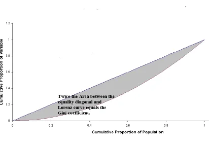
The Gini coefficient is derived from the Lorenz Curve (Ceriani and Verme, 2012). The Lorenz curve has been used extensively in studying income distribution. To plot a Lorenz curve, rank the observations from lowest income to highest income or the variable of interest. Then plot the cumulative proportion of the population on the horizontal axis and the cumulative proportion of the variable of interest on the vertical axis (Figure 3.1). The Gini coefficient compares this cumulative frequency curve to the uniform distribution that represents equality. In Figure 3.1 below, the diagonal line represents perfect equality. The greater the deviation of the Lorenz urve from this diagonal line, the greater the inequality. The Gini coefficient is defined as the ratio of the areas in the Lorenz curve. Let the area between the equality line and the Lorenz curve be denoted by A, and the area under the Lorenz curve by B. Then the Gini coefficient is given by A/(A+B). If the area of the rectangle is taken as 1, then A+B = 0.5. This implies that the Gini coefficient is 2A that is double the area between the equality line and the Lorenz curve.

23

Figure 3.1: Lorenz Curve

Ceriani and Verme (2012).

Let N be the total number of individuals in all the classes, with Ni of these belonging to the ith

class, i = 1, 2, . . . , g. The Gini index (also known as Gini impurity measure), at node t denoted by G (t), is given by

 

j i

ip

p t

G



 

Where pi is the probability that an individual belongs to the ith class.

24













This is commonly referred to as the Gini index.

Suppose the data is split using a splitting criteria, into two subnode t1 and t2 with sizes N1 and N2

respectively. The Gini index of the split data is given by;

 

 

 

 

Ginisplit   (3.4)

The following procedure is used to select the splitting variable and the splitting value.

i. Choose a variable and a value and split the node. Calculate the Gin isplit (t).

Repeat this over all possible variables at the node.

ii. Select the variable and the value with the least Ginispli t and use it for splitting. It

is known as the splitting variable.

iii. Repeat this process at each node until splitting is completely done. (Breiman et al., 1984)

3.3.2 Pearson’s chi –squared statistic

Suppose there are g independent classes. Let N be the total number of individuals with Ni

25

After a set of splits have been decided, a goodness of fit test is performed to select the best split. A split that makes the two subnodes as pure as possible (most heterogeneous) is the best split. We may define the hypothesis as:

H0: the population proportions are the same in the right and left subtrees after the split.

H0 is the most homogeneous tree. However the best split gives the most heterogeneous tree.

Therefore, the best split is the one in which Ho is rejected. Therefore a statistic that tests for the homogeneity of a g × 2 contingency table is a suitable test statistic.

The statistic;









i j ij ij ij

E E

O 2

2



(3.5)

is used to for homogeneity in the contingency tables;

where Oij = Nij are the observed frequencies and

N N N

E_ij  i j are the estimated expected

frequencies.

The variable and value that maximizes the χ2

is the one that gives the most heterogeneous split. Therefore this is the best value and variable to use in the splitting.

26

 Calculate the Pearson’s Chi-Squared value among the child branches over all possible

points for each variable Xh at each node. h = 1, 2, . . . , k

 Select the variable and the value of that variable with the maximum chi-squared statistic

value, denoted by Xh0 and use it for splitting.

Repeat this process at each node until splitting is completely done. The theoretical basis of the Chi-Square distribution in (3.5) is given in theorem 3.1.

Theorem 3.1









i j ij

ij ij E E O 2 2

 Converges in distribution to the chi-square distribution.

Proof

A sequence of random variables {Xn} is said to converge in distribution to a random variable X

if

 









 

at each continuity point x of F(x).

Let



  n l l X 1  

 be the number of observations in the αth

class (the observed frequency in the

αth

class). Let pα be the probability of an individual belonging to class α. Then the expected

27 Let











Define p_ q_,  1,2,,k

Let             k q q q      0 0 1 Then q k q q q 1 1 1 1 0 0 1                        (3.8)

Let 

     _   _    p n n n

28                           _       _       _               k k kn n n n p n n p n n p n n          2 2 1 1 2 1 (3.9)

If we let

29 n q q n n q n q n n k n n q T           1 1 ' 1 1 ' 2 1 2                                



 is obtained as follows

                                                                  _       _                                   _       _       _              









Now x1 





30









 

 

 





E _l  _l2  _l  1

For



 



Cov _{l l l l}

     , Now n l x x x x X lk l l l l    , 2 , 1 2 1                       

Are independently and identically distributed random variables with mean vector

             k p p p  2 1 

and covariance matrix













 k k k

31

By the Central Limit Theorem, L

 

 

That is is degenerate Nk (0,Σ). It then follows that L

 

 

q q

n 

                   

 1 1

Where 

q

V ₁ is degenerate _

        q q k

N 0, 1 1 .

Therefore,

Where Vis degenerate _

         q q k

N 0, 1 1 .

Then,

(3.14)

Where z1, z2, . . .,zk are independent normal random variables and λ1, λ2, . . . , λk are the

characteristic roots of _

         q q 1

1 . We assume that 

         q q 1

1 has characteristic root 1

with multiplicity k-1 and 0 with multiplicity 1. It follows that;

.

 









n n

n     

' 2

 

 



n LVV L z

T L

1 2

2 

 





32

3.3.3 Gain ratio

This impurity measure uses the information provided by the attribute. It represents the potential information generated by splitting data into n partitions. Information theory measures information content by use of bits. One bit of information is enough to answer a yes or no question. If the possible answers vi have probabilities P(vi), then the information content I ( or

information gain) of the actual answer is given by;

 



   

 



 

 

i

i

n

v P v

P

v P v

P v P I t Gain n Informatio

2 1

2 1

log , . . . , ,



  



(3.15)

The higher the information gain, the better the splitting variable(Shannon and Weaver, 1964).

Suppose we have a set of possible events whose probabilities of occurrence are p1, p2, . .., pn.

These probabilities are known but that is all we know concerning which event will occur. The problem is to find a measure of how much "choice" is involved in the selection of the event. This is equivalent to finding how uncertain we are of the outcome. If such a measure exists, say H(pI,

p2,.,pn), it has the following properties:

1. H should be continuous in the pi.

2. If all the pi are equal, pi= 1/n then H should be a monotonic increasing function of n. With

equally likely events there is more choice, or uncertainty, when there are more possible events.

33

Theorem 3.2(Shannon and Weaver, 1964)

The only H satisfying the three assumptions above is of the form:

i i

i p

p K

H 



Where K is a positive constant.

Proof

Let A

 

n n

H  

  



 1

. , 1 , 1



From condition (3) above, we can decompose a choice from Sm equally likely possibilities to a series of m choices from S likely possibilities and obtain

 

 

A m 

Similarly

 

 

A n 

We can choose an n arbitrarily large and find an m to satisfy

1

 

 n m

m

S t S

Taking logarithms we get





t n S

mlog2  log2  1log2

34 n n m S t n m 1 log log 2

2  



This is equivalent to

         S t n m 2 2 log log

Where ε is an arbitrary small number.

From the monotonic property of A(n), it follows that,

     

S A t A S A That is

 

 





 

mA   1

Dividing throughout by nA(S) we obtain

 

35

 

 

log log 2 2         S t S A t A

Let A(t) = -Klogt (where K is a positive constant chosen to satisfy condition 2).

Now suppose we have a choice from n possibilities with commeasurable probabilities



p where the ni are integers. We can break down a choice from



choice from n possibilities with probabilities p1,..., pn. Using condition 3 again, we equate the

total choice from







i H p p p K p n

n

Klog₂





This implies that,



_





_



 

Without loss of generality, take K = 1 to obtain,

i

i p

p H 



36

Let Ni be the number of individuals allocated to branch i and let N denote the total number of

individuals. Then the intrinsic information at node t is given by;

Intrinsic Information(t) = _N N N

Ni i

2

log



(3.16)

The gain ratio at node t is given by,

 

 

_{ }

t n Informatio Intrinsic

t Gain n Informatio t

Ratio

Gain 

(3.17)

The following procedure is used to select the splitting variable and the splitting value.

i. Work out the Information Gain among the child branches over all possible decision points for each variable Xj at each node.

ii. Select the variables and the values of these variables with Information Gain that is neither too small nor too large.

iii. Work out the Gain Ratio among the child branches selected in (ii) above

3.4 Testing for Differences in Performance among the Trees

To compare the performance of the trees, the McNemar’s test procedure is used. The McNemar’s test procedure is used to determine which of two classifiers, C1 and C2 say, has lower error rate

(Lindgren, 1993). The procedure is as follows:

Run the two classifiers on data set and record the following information

37

n11: the number of individuals misclassified by both.

n01: the number of individuals correctly classified by C1 but misclassified by C2.

n10: the number of individuals correctly classified by C2 but misclassified by C1.

Define the statistic M as follows that,





10 01

2 10

01 1

n n

n n M

  

 (3.18)

38

CHAPTER FOUR

COMPARISON OF CRISP AND FUZZY CLASSIFICATION USING

DIFFERENT IMPURITY MEASURES

4.1 Introduction

In this chapter, fuzzy and crisp classification trees were compared. The fuzzy tree was constructed using triangular membership function. The probabilities of correct allocation were then calculated. Comparison of the performance of fuzzy tree with crisp tree was carried out using simulated data and then applied to real data. The first set of observations was generated from two 3-variate normal populations with different mean vectors but a common dispersion matrix. The second set of observations was generated from three 4-variate normal populations with different mean vectors but a common dispersion matrix. Simulated data was obtained using R statistical package and implemented on Pentium IV running on Windows 7 environment. The two sets of real data that were used in the study came from UCI machine learning repository.

4.2 Results from 3-variate normal populations based on simulated data

39

probabilities of correct allocation, P11 and P22 for both crisp and fuzzy classification trees. Table

40

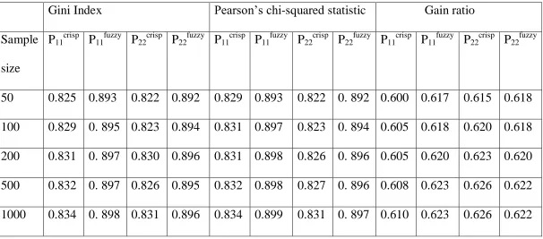
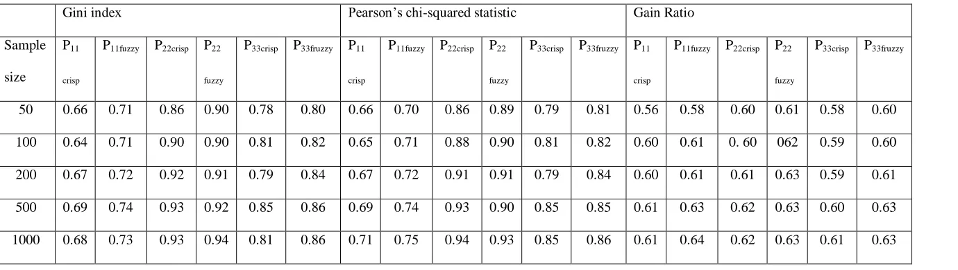
Table 4.1: Probabilities of Correct Allocation for Gini Index, Pearson’s Chi-squared Statistic and Gain Ratio

Gini Index

Pearson’s chi-squared statistic Gain ratio

Sample

size

P

P

P

P

P

P

P

P

P

P

P

P

41

From table 4.1 it was noted that the average probabilities of correct allocation using fuzzy trees are generally higher than the probabilities of correct allocation when crisp trees are used. This was true for the three impurity measures considered in the study. Correct probabilities calculated for the Gini Index and the Pearson’s chi-squared statistic are comparable. However those for gain ratio are much lower than for the other two. Therefore gain ratio did not perform as well as the other two impurity measures for this type of data.

It was also noted that as the sample size increased, the probabilities of correct allocation marginally increased both for the crisp and fuzzy classification trees.

The proportion of times probabilities of correct allocation was higher when using crisp cut points than fuzzy decision points is given in table 4.2.

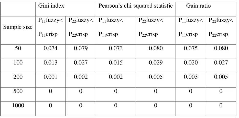
Table 4.2: Proportion of times crisp probabilities outperforms fuzzy probabilities Gini index Pearson’s chi-squared statistic Gain ratio

Sample size

P11fuzzy<

P11crisp

P22fuzzy<

P22crisp

P11fuzzy<

P11crisp

P22fuzzy<

P22crisp

P11fuzzy<

P11crisp

P22fuzzy<

P22crisp

50 0.074 0.079 0.073 0.080 0.075 0.080

100 0.013 0.027 0.015 0.029 0.020 0.027

200 0.001 0.002 0.002 0.005 0.003 0.005

500 0 0 0 0 0 0

42

From table 4.2, we note that the proportion of times the crisp classification tree outperformed the fuzzy classification tree was very low. This is true for the three impurity measures. Therefore one can conclude that the fuzzy classification tree performs better than crisp classification tree for these data.

4.2.1 Testing for difference in performance of the impurity measures for simulated data

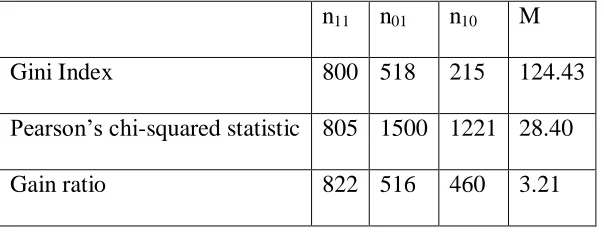
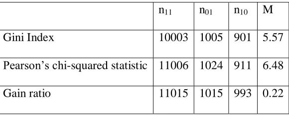
The values of n11, n01 and n10for the three impurity measures are given in Table 4.3, C1 is taken

as fuzzy classification tree and C2 as crisp classification tree. The McNemar’s value in equation

3.10 is calculated and compared to the tabulated chi-squared value at 95% confidence.

Table 4.3:McNemarsValues for Gini Index, Pearson’s Chi-squared statistic and Gain Ratio n11 n01 n10 M

Gini Index 800 518 215 124.43

Pearson’s chi-squared statistic 805 1500 1221 28.40

Gain ratio 822 516 460 3.21

At 95% confidence level and p-value of 0.1056, ₁2_,0.95= 3.84. Since both 28.40 and 124.43 are

43

4.2.2 Different Sample Sizes of population one and population two from the 3-variate normal populations simulated data

44

Table 4.4a: Probability of correct allocation to population one for different combinations sample sizes

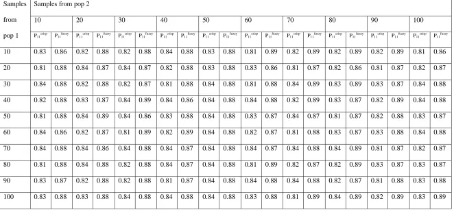
Samples from pop 1

Samples from pop 2

10 20 30 40 50 60 70 80 90 100

P11crisp P11fuzzy P11crisp P11fuzzy P11crisp P11fuzzy P11crisp P11fuzzy P11crisp P11fuzzy P11crisp P11fuzzy P11crisp P11fuzzy P11crisp P11fuzzy P11crisp P11fuzzy P11crisp P11fuzzy

45

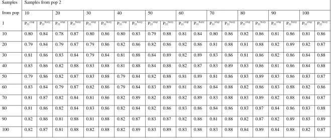
Table 4.4b: Probability of correct allocation to population two for different combinations of sample sizes

Samples

from pop

1

Samples from pop 2

10 20 30 40 50 60 70 80 90 100

P22crisp P22fuzzy P22crisp P22fuzzy P22crisp P22fuzzy P22crisp P22fuzzy P22crisp P22fuzzy P22crisp P22fuzzy P22crisp P22fuzzy P22crisp P22fuzzy P22crisp P22fuzzy P22crisp P22fuzzy

10 0.80 0.84 0.78 0.87 0.80 0.86 0.80 0.83 0.79 0.88 0.81 0.84 0.80 0.86 0.82 0.86 0.81 0.86 0.81 0.86

20 0.79 0.84 0.79 0.87 0.79 0.86 0.82 0.86 0.82 0.86 0.82 0.86 0.81 0.88 0.81 0.88 0.82 0.89 0.82 0.87

30 0.81 0.86 0.83 0.84 0.79 0.84 0.81 0.88 0.84 0.89 0.82 0.89 0.83 0.86 0.81 0.86 0.82 0.86 0.84 0.88

40 0.83 0.86 0.82 0.88 0.83 0.88 0.81 0.88 0.84 0.88 0.82 0.87 0.83 0.89 0.83 0.86 0.81 0.86 0.84 0.88

50 0.79 0.86 0.82 0.87 0.83 0.88 0.79 0.84 0.82 0.88 0.81 0.89 0.81 0.86 0.83 0.89 0.83 0.86 0.83 0.87

60 0.83 0.84 0.79 0.87 0.82 0.86 0.79 0.84 0.83 0.89 0.81 0.86 0.84 0.88 0.82 0.86 0.83 0.88 0.82 0.86

70 0.81 0.87 0.82 0.84 0.81 0.86 0.82 0.89 0.82 0.88 0.82 0.89 0.83 0.88 0.83 0.89 0.82 0.88 0.84 0.87

80 0.81 0.86 0.82 0.84 0.83 0.86 0.82 0.84 0.82 0.86 0.83 0.86 0.84 0.86 0.83 0.87 0.84 0.86 0.83 0.88

90 0.82 0.86 0.81 0.88 0.81 0.88 0.82 0.87 0.83 0.87 0.82 0.86 0.81 0.88 0.82 0.87 0.82 0.89 0.83 0.89

46

From tables 4.4a and 4.4b it is noted that there is no difference in the values of probabilities of correct allocation even with different sample sizes in the two populations. Hence one can conclude that for both crisp and fuzzy classification trees sample size difference does not affect the performance of either fuzzy or crisp classification trees.

4.3 Results from 3-variate normal populations based on real data

This set of data was for measurements of tortoise shells from UCI machine learning repository. The first population was from 500 female tortoise and the second population was from 500 male tortoise. X1 denotes the shell length, X2 the shell width and X3 the shell height. All the

measurements were in millimeters. It was assumed that the populations are normally distributed with different means but same dispersion matrix. From the data, the sample mean vectors and pooled sample variance matrix are given as:

1 2

113.4 136.0

88.3 102.6

40.7 52.0

282.8 167.9 98.8 167.9 106.2 59.9 98.8 59.9 37.3

u

X X

S

   

   

_{ } _{ }

   

   

 

 

  

 

 

Where

1

X is the sample mean vector from population one ( female tortoise)

2

X is the sample mean vector from population two (male tortoise)

47

The splitting value that was selected for each variable was the mean value of the combined samples. Both crisp and fuzzy classification trees were used. To generate the tree one-third of the instances were used and the rest two-thirds were used to test the tree performance. This was done by calculating the probabilities of correct allocation.

Shell Length

For fuzzy cut points, the peak is taken as the mean of the shell length, with left width one standard deviation and right width one standard deviation.

From the sample mean vectors and the combined sample variance matrix above, the mean shell length is 124.7mm and the variance of shell length is 282.8mm2, giving a standard deviation of 16.8mm.

For fuzzy classification tree, any tortoise with shell length, x, less than 124.7mm was allocated to the left branch. If x is greater than 124.7mm, the tortoise was allocated to the left branch with probability p(x), where;

 

     

   

 

5 . 141 ,

0

5 . 141 7

. 124 8

. 16

7 . 124 1

x x x

x

p (see definition 1.3)

48

Shell width

For fuzzy cut points, the peak is taken as the mean of the shell width, with left width one standard deviation and right width one standard deviation.

The mean shell width is 95.4mm and the variance of shell width is 106.2 mm, giving a standard deviation of 10.3mm.

For fuzzy classification tree, any tortoise with shell width, x, less than 95.4mm was allocated to the left branch. If x is greater than 95.4mm, the tortoise was allocated to the left branch with probability p(x), where;

 

     

  

 

7 . 105 ,

0

7 . 105 4

. 95 , 3 . 10

4 . 95 1

x x x

x

p (see definition 1.3)

For crisp classification trees, any tortoise with shell width of 95.4mm was allocated to left branch with probability one, otherwise it was allocated to the right branch.

Shell height

For fuzzy cut points, the peak is taken as the mean of the shell height, with left width one standard deviation and right width one standard deviation.

49

For fuzzy classification tree, any tortoise with shell height x, less than 46.35 mm was allocated to the left branch. If x is greater than 46.35mm, the tortoise was allocated to the left branch with probability p(x), where;

 

p (see definition 1.3)

For crisp classification trees, any tortoise with shell height of 46.35mm was allocated to left branch with probability one, otherwise it was allocated to the right branch.

Using the above allocation criteria, the results in Table 4.5 were obtained.

Table4.5: Instances Individuals Are Allocated to Right and Left Branches

Crisp results Fuzzy results

Sample from

Population 1 (Female Tortoise) Shell length Shell width Shell height Shell length Shell width Shell height

left 350 400 440 357 403 446

right 150 100 60 143 97 54

total 500 500 500 500 500 500

Sample from

Population 2 (Male Tortoise)

left 100 130 54 88 127 54

right 400 370 446 412 373 446

total 500 500 500 500 500 500

50

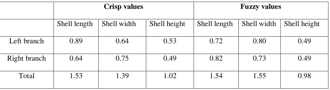
Table 4.6a: Information Gain calculated Values

Crisp values Fuzzy values

Shell length Shell width Shell height Shell length Shell width Shell height

Left branch 0.89 0.64 0.53 0.72 0.80 0.49

Right branch 0.64 0.75 0.49 0.82 0.73 0.49

Total 1.53 1.39 1.02 1.54 1.55 0.98

Table 4.6b:Intrinsic information calculated values

Intrinsic Information Shell length Shell width Shell height Crisp values 0.992 0.997 1.00

Fuzzy values 0.999 0.997 1.00

Table 4.6c: Gini Index, Pearson’s Chi-Squared and Gain Ratio calculated values Crisp decision point values Fuzzy decision point values

Shell length Shell width Shell height Shell length Shell width Shell height

Gini index 0.360 0.348 0.215 0.353 0.305 0.193

Pearson’s Chi-squared statistic

614.7 305.8 293.3 640 355 193

Gain ratio 1.54 1.39 1.02 1.55 1.12 0.98

51

therefore shell height was used as the splitting variable at about 46.35mm. For both crisp and fuzzy trees while applying the Gin index, shell height was used.

For Pearson’s chi-square statistic, shell length has the maximum value both crisp and fuzzy trees. Therefore shell length at 124.7mm was used as the split variable when applying the Pearson’s chi-square statistic.

The Gain ratio had maximum value for shell length at 124.7mm. Therefore shell length was used as the split variable.

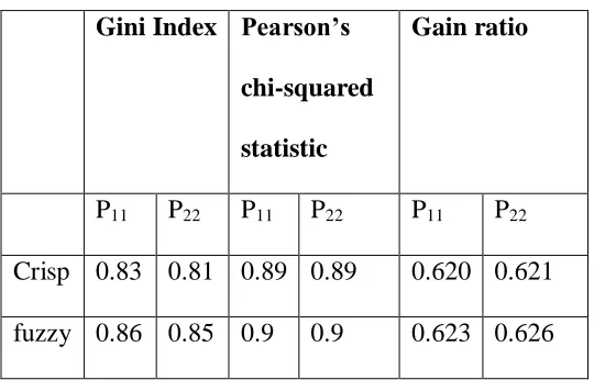
In classifying allocate left branch to population one (female tortoise) and right branch to population two (male tortoise). Using this allocation rule, classification was done using the rest of the data and the probabilities of correct allocation were calculated by applying the Gini index, Pearson’s chi-square statistic and the Gain ratio.

Table 4.7: Probabilities of correct allocation Gini Index Pearson’s

chi-squared statistic

Gain ratio

P11 P22 P11 P22 P11 P22

Crisp 0.83 0.81 0.89 0.89 0.620 0.621 fuzzy 0.86 0.85 0.9 0.9 0.623 0.626

52

4.3.1 Testing for difference in performance of the impurity measures for real data

Table 4.8McNemars values for real data

n11 n01 n10 M

Gini Index 100 8 14 1.14

Pearson’s chi-squared statistic 102 10 14 0.375

Gain ratio 105 3 7 0.43

It was found out (Table 4.8) that for the three impurity measures, the calculated M values were

smaller than

2 95 . 0 , 1



= 3.84. Therefore at 95% confidence and p-value of 0.112, we conclude that, there was no difference between the crisp classification tree and the fuzzy classification trees.

4.4 Results from 4-variate normal populations based on simulated data

This set of data was from three 4-variate normal populations with different mean vectors and common dispersion matrix. From each of the three populations 5000 samples were generated. 1000 samples out of the 5000 were used to create the trees. The remaining 4000 samples from each population were used to test the trees. The probabilities of correct allocation, P11, P22 and

P33 were calculated. This was done for the crisp and fuzzy decision points.

53

Table 4.9: Probabilities of Correct Allocation using simulated data

Gini index Pearson’s chi-squared statistic Gain Ratio Sample

size

P11 crisp

P11fuzzy P22crisp P22 fuzzy

P33crisp P33fruzzy P11 crisp

P11fuzzy P22crisp P22 fuzzy

P33crisp P33fruzzy P11 crisp

P11fuzzy P22crisp P22 fuzzy

P33crisp P33fruzzy