NOTE ON GENETIC DRIFT AND ESTIMATION OF EFFECTIVE POPULATION SIZE

Letter

to the Editor

N O T E O N GENETIC D R I F T

A N D

E S T I M A T I O N O F

EFFECTIVE P O P U L A T I O N SIZE

Recently POL.LAK (1 983) proposed a new method for estimating the effective population size from allele frequency changes and compared his method with NEI and TAJIMA’S (1981) method. Although both methods are very similar, the former uses

as a measure of standardized variance of gene frequency changes for a locus, whereas the latter uses

where K is the number of alleles, and x, and

y,

are the observed frequencies of the ith allele in the 0th and tth generations, respectively. When there are data from different loci, weighted means of F K I and F,, i.e., F K I = 2,(KJ

-

l)FKI,/

Z,(K,

-

1) and F, = Z,K,F,/ZK,, are used, where subscript j refers to the j t h locus. Once FK1 or F, is obtained, the effective size is estimated by formula (16) or (1 8) in NEI and TAJIMA (198 1).

In this connection it should be noted that in NEI and TAJIMA’S (1 98 1) definition of F,, K

-

1 is used in place of K . In their computation, however, K F,’s are first computed by eliminating one allele at a time from allele A1 to allele AK, and the average is used as the final value of F,. This average is equal to ( 2 ) . For example, in the case of three alleles, we can compute three Fr’s, i.e., Fr12 = (F,1

+

F c 2 ) / 2 , Fr13 = (F,1

+

Fc3)/2 and Fr23 = (Fr2

+

Fr3)/2, where Fa = (x,

-

yJ2/[(xi

+

y J / 2

-

x,!;]. T h e average is

Fc = (Fr12

+

Fc13

+

Fc23)/3

= (Fc1

+

Fr2

+

Fr3)/3.

This shows that NEI and TAJIMA’S F, is identical with

(2).

However, note that the number of degrees of freedom for computing the

x 2

is K

-

1 rather than K .

At any rate, when he compared (1) and ( 2 ) , POLLAK (1 983) concluded that F,

is superior to F K l for K = 2 but inferior for K 2 3. This conclusion is based on the following observations. (1) T h e expectation of FK1 is approximately equal to that of F,. ( 2 ) T h e maximum value of FK1 is 4 / ( K

-

l), whereas that of F, is 2 . ( 3 ) When K = 2 . the variance of F, is approximately equal to that of F K ~ . (4) T h e

570 F. TAJIMA AND M. NE1

variance of F K I is smaller than that of F, when the initial frequencies vary substantially with K 2 3. However, his formulations involve some approximations. In this note w e show that observations ( 2 ) and (3) are incorrect and present more accurate formulas for the variances of F K ~ and F,.

Equation

(2)

can be written as

&J(2

-

X I

-

yJ

xr

+

Jl

-

2x*y,

K

,=1 (3)

Thus, the maximum value of F , is 4 / K , which is always smaller than that

[ 4 / ( K

-

I)] 0fF.u.

In order to obtain the variances of FK1 and F,, POLLAK (1983) considered the variance of the numerator of (1) or

(2),

but ignored the variance of the denom- inator and the covariance between the numerator and denominator. H e did this because he was interested in the case of relatively large sample sizes. When sample sizes are small, however, we must consider all of these components. (When gene frequency data for many different alleles or loci are used, even a small sample size gives a fairly reliable estimate of IV.) In this case the variance of F K 1 becomes

approximately, where

p ,

is the frequency of the ith allele in the population at generation 0, and F and G are quantities dependent on the sampling scheme used. If we use sampling scheme I of NEI and TAJIMA (1 98 l ) , they become

1 1 t - 2

2so

2s, 2*v '

F = - + - + -

3 t

-

1 ( t

-

1)(3t - 4 )

2

G =

+

where SO and S , are the sample sizes in the 0th and tth generations, respectively, and IV is the effective population size. In their sampling scheme I1 we have

1 1 t

F = - + - + -

2so

2s,

2 N '

LETTER TO THE EDITOR 571

-

+

-

in sampling scheme 11. T h e moments of gene frequency changes

necessary for obtaining (4) and ( 5 ) are given by NEI and TAJIMA (1 98 1) and POLLAK

(1983), except the following ones [ c j , pp. 332-335 in CROW and KIMURA (1 970)].

(2:, 2;)

-

pJ3

+

( y t

-

P J ~ I

=

PO

-

p&l

-

2 p , ) ~ ,

E[(.r,

-

pi)2(xi

-

p j )

+

(4’1

-

pr)2(J~

-

p ~ ) ]

ptpj(2pt

-

1)G.

Before we compare V(Fc) with v ( F K I ) , let us examine the accuracies of (4) and

( 5 ) , since these equations still involve some approximations. For this purpose, we

use the results obtained from a computer simulation by NEI and TAJIMA (1981)

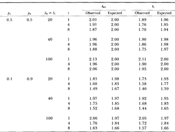
for sampling scheme I. We compare the quantities defined as

~ K I = ( K

-

I ) V ( F K I ) / [ E ( F K I ) ] * ,

k r = ( K

-

1)V(Fr)/[E(Fr)]*.

( 6 4

(6b)

T h e observed values of (6a) and (6b) obtained from the computer simulation and the expected values from

(4)

and ( 5 ) are presented in Table 1. There are some differences between the expected and observed values. However, if we note that in POLLAK’S (1983) formulas kKI = k, =

2

for all cases of K = 2 , the

expected values obtained from

(4)

and ( 5 ) are much closer to the observed values than POLLAK’S. Particularly when

p ,

deviates from 0.5 or when t is large, (4) and

( 5 ) give much better values of k K 1 and k, than POLLAK’S formulas.

Table 1 also shows that, unlike POLLAK’S conclusion,

k,

is always smaller than or equal to

k K 1

when K = 2. Since the expectations of F, and F K I are more or less the same, this indicates that F, is a better quantity than F K 1 for estimating effective population size. When K 2 3 ,

k,

is again smaller than k K 1 if

p,

= 1 / K .

This is because, in this case,

V(FK1)

and V(Fc) become

V(FK1) 2 F 2 / ( K

-

l ) ,

V(F,) 2F(F

-

2 H ) / ( K

-

1).

Therefore, V(F,)

<

V(FK1).

When the initial frequencies vary considerably, however, k, is usually slightly larger than k ~ 1 . Several examples for K = 3 are shown in Table 2. Therefore, POLLAK’S observation

(4)

seems to be correct.

From this study, we can conclude that when a majority of loci studied have only two alleles, F, is preferable to F K ] . If a majority of loci have more than two alleles and their frequencies deviate from 1/K considerably, then FKI is slightly

better than F,. In any case, however, the difference between the variances of F K l

and F, i s very small, so that both methods can be used.

In this connection BRUCE WEIR has suggested that the following quantity ( F d ) , which is equivalent to LATTER’S (1973)

4*,

might give a better estimate of AT

572 F. TAJIMA AND M. NE1

-

t Observed Expected

2.00 2.00 2.00

Observed Expected

1.89 1.96

1.76 1.95

1.70 1.94

-

Pl P 2 so = s,

0.5 0.5 20 1

4

8

2.01 1.91 1.87

40 1

4 8 1.96 1.96 1.88 2.00 2.00 2.00

1.90 1.98 1.86 1.98 1.75 I .97

100 1

4 8 2.13 1.96 2.06 2.00 2.00 2.00

2.11 2.00 1.90 2.00 1.95 2.00

0.1 0.9 20 1

4 8 1.83 1.68 1.49 1.98 1.83 1.67

1.73 1.93 1.58 1.77

1.40 1.59

40 1

4 8 1.97 1.75 1.52 1.97 1.85 1.68

1.92 1.95

1.68 1.83

1.44 1.65

100 2.06

1.76 1.63

1.97 1.84 1.66

2.05 1.97

1.72 1.84

1.57 1.66

1

4 8

Observed values were obtained from NEI and TAJIMA’S (1981) computer simulation. iV = 100

and K = 2 are assumed.

T A B L E 2

Thpowticrrl artlues of k,,, k, roid kd

so = s, = 100 1v= 1000

s o = s, = 20

’\’ = 100 Sampling

P. p. scheme

__

1/3 1/3 I

I 1

k K I k, k d

2.00 1.99 1.99 2.00 1.99 1.99

k, k d

1.94 1.94 1.93 1.93

_ _

2.00 2.00

0.2 0.3 0.5 I

I1

2.00 2.02 2.11 2.00 2.02 2.11

1.97 1.97

1.95 2.05 1.93 2.03

1.99 2.07 2.56 1.98 2.07 2.55

0. I 0.4 0.5 I

I1

1.87 1.86

1.96 2.48 1.94 2.46

0. I 0.1 0.8 I I1

1.97 2.09 2.30 1.96 2.09 2.29

1.72 1.69

1.81 2.02 1.77 1.98

L E I T E R rO T H E EDITOR 573

K K

Fd =

c

(st - J ? ) Z /

c

[(xt

+

JJ/2

- XrJt].

(7)

1=1 r=l

This is because REYNOLDS, WEIR and COCKERHAM'S (1 983) computer simulation has shown that this gives a less biased estimate of inbreeding coefficient than F, when

p,

deviates from 1/K and t is large. However, the theoretical variance of

F,, has not been determined. We have, therefore, derived a formula for this variance, which is given by

T h e numerical values of k d = (K

-

l)V(Fd)/[E(Fd)]' in comparison with kK1 and

k, are given in Table

2.

When

p,

= 1/K, k d is virtually the same as k,. However, as

I,

deviates from 1/K, k d becomes larger than k,, and the difference can be substantial. This is in agreement with the results of REYNOLDS, WEIR and COCKERHAM (1983) from computer simulation, in which V(Fd) was shown to be considerably larger than V(F,), although the smaller bias of F d resulted in a smaller mean squared error for Fd than for F,. (Simulation of REYNOLDS, WEIR and COCKERHAM also shows that, for t = 20 and K =

2,

V(Fd) is smaller than

V(FK1) when

fi,

= 0.5 but larger than V(FK1) when

pi

deviates from 0.5 consider- ably.) This result is in agreement with our theoretical prediction. Note that the

t of REYNOLDS, WEIR and COCKERHAM corresponds to our 2t because they considered two populations rather than one.) We can, therefore, conclude that F, is better than Fd from this point of view. It should also be noted that in the case of estimation of effective population size the t value used is generally small (about 10 or less), and, in this case, the bias of the estimate of F obtained from F, is very small even if

p ,

deviates considerably from 1/K (see Table 3 of NEI and TAJIMA 1981). Furthermore, F, has the advantage that it is approximately distributed as a

x2

variate, so that the confidence interval of the estimate of

,\'

can easily be estimated. If we consider all these factors, F, seems to be better than Fd.

LITERATURE CITED

CROW,J. F. and M. KIMURA, 1970 A H Introduction toPopulation Genetics Theory Harper & R o w , New

LATTER, B. D. H., 1973 Measures of genetic distance between individuals and populations. pp. 27- 39. In: Genetir Structure of Poptclntions, Edited by N. E. MORTON. University Press of Hawaii, Honolulu, Hawaii.

Genetic drift and estimation of effective population size. Genetics 98:

A new method for estimating the population size from allele frequency changes. York.

NEI, M . and F. TAJIMA, 1981

POLLAK, E., 1983

625-640.

5 74

REYNOLDS, J., B. S. WEIR and C. C. COCKERHAM, 1983 F. TAJIMA AND M. NE1

Estimation o f the coancestry coefficient: basis for a short-term genetic distance. Genetics 105: 767-779.

FUMIO TAJIMA and MASATOSHI NEI

Center for Demographic and Population Genetics The University of Texas at Houston