Reliability and Availability Analysis of a Dissimilar Unit Cold Standby System withMaximum Redundancy Time Limit

2636 | P a g e

Reliability and Availability Analysis of a Dissimilar Unit

Cold Standby System withMaximum Redundancy Time

Limit

R.K. Bhardwaj, Komaldeep Kaur

Department of Statistics, Punjabi University Patiala-147002, India

ABSTRACT

A probabilistic model of a cold standby system is developed. There are two dissimilar units in the system.

Initially the system starts operating taking original unit in active and duplicate in passive mode. The passive unit

fails after crossing a pre-specified time limit and become degraded after repair. The theory of renewal processes

is explored to derive expressions for reliability and availability of the model. An assumed data set is considered

for numerical analysis of the results. For a special case all the random variables are assumed to follow Weibull

distribution.

Keywords

-

Availability, Reliability, Redundancy Time, Standby System, Stochastic Processes.

1.

INTRODUCTION

The reliability and availability are the vital characteristics of a working system.There are various ways to

improve theseessentials attributes. To serve this cause some redundancy techniques are discussed in the related

studies. The cold standby redundancy is one such techniqueused commonly in the literature [1-6]. Most of the

studies considered identical units for the standby [7-14]. This consideration seems costlier as the standard unit

always has budgets higher than a duplicate unit.

Therefore, keeping this fact in view in this paper a dissimilar unit cold standby system models is

considered.To save cost a duplicate unit is taken as standby instead of a standard one. As the original unit fails it

goes under repair and becomes as new after each repair. The duplicate standby unit can fails after exceeding a

pre-specified maximum time limit, termed as maximum redundancy time limit.There is a single repair facility in

the system,accountable for all remedial actions. The duplicate unit becomes degraded after the first repair and

gets replaced by new one at further failure. The replacement takes some random amount of time andthe original

unit is given the first choice for operation as well as repair upon the duplicate unit.All the random variables are

statistically independent and follow general probability distribution with distinct distribution functions. The

inter-switching of original and duplicate unit is perfect and prompt. The paper utilized the concepts of

semi-Markov regenerative processes of renewal theory [15-17]. The expressions are derived for reliability and

availability of the system.An assumed rough data set is taken for the numerical exploration of results.For the

2637 | P a g e

2.

NOTATIONS

E

E/ : The set of regenerative/ Non-regenerative states

2 2 1

No

Do

No

: Original unit/ Duplicate unit/ Degraded unit in operation. 2

2

DCs

Cs

: Duplicate unit/ Degraded unit in cold-standby mode.

i

i UR

ur F

F : Failed unit i= 1, 2 under repair /under repair continuously from previous state.

2

2 WR

wr F

F : Duplicate failed unit waiting for repair / waiting for repair continuously from previous

state.

2

2 URp

urp DF

DF : Degraded failed unit under replacement / under replacement continuously from previous

state.

2

2 WRp

wrp DF

DF : Failed unit waiting for replacement / waiting for replacement continuously from

previous state.

) ( / ) (t Z t

z_{i i} : pdf / cdf of failure time of i= 1, 2 unit.

) ( / )

( ₂

2 t Z t

z_{d d} : pdf / cdf of failure time of degraded unit.

) ( / )

( ₂

2 t S t

s : pdf / cdf of maximum redundancy time of duplicate unit.

) ( / )

( ₂

2 t S t

s_{d d} : pdf / cdf of maximum redundancy time of degraded unit.

) ( / ) (t G t g

i

i : pdf / cdf of repair time of i=1, 2 unit.

) ( / ) (

2

2 t F t

f

d

d : pdf / cdf of replacement time of degraded unit.

) ( ) (t Q t

q_{ij ij} : pdf/cdf of first passage time from regenerative state i

S to regenerative State S_j or

failed state S_j without visiting any other regenerative state in



0,t



.

) ( ) (

.

. t Q t

q

kr ij kr

ij : pdf/cdf of first passage time from regenerative state Si to regenerative state Sj or failed

state S_j visiting state k

S ,

S

_r once in



0,t



.

)

(

t

i



: Probability that the system up initially in state S_iEis up at time t without visiting to

any regenerative state

) (t

W_i : Probability that server busy in the state i

S up to time t without making any transition

to any other regenerative state or returning to the same state via one or more

non-regenerative states

] /[ ]

[s c : Symbol for Laplace-Stietjes convolution/Laplace convolution

/*

~ : Symbol for Laplace- stietjes Transform (LST)/Laplace transform (LT)

) (

2638 | P a g e

3.

THE MODEL DEVELOPMENT

The following are possible transition states of the system model

The regenerative states:



,



,

2 1 0 No Cs

S 















₂

1

F

₁

,

No

S

_ur ,















2

,

1 2

No

F

ur

S

,



,



,

2 1 3 No DCs

S  ₄_ , ₂_

1

Do F

S _ur ,















2

,

1 5

No

DF

urp

S

The non-regenerative states:

,

,

2 1

6















F

_UR

F

_wr

S

_ _

2 1

,

7 Fur Fwr

S ,















2 1

,

8

F

UR

DF

wrp

S

, 

      2 1 ,

9 Fur DFwrp

S

3.1 Transition Probabilities and Mean Sojourn Times

Simple probabilistic considerations yield the following expressions for the non-zero

elements:- 

_



 

   0 dt t q Q

p _{ij ij}

ij (1)







 



    



0 2 1

16

0 1 2

10

0 1 2 02 0 2 1

01 z (t)S (t)dt, p s (t)Z (t)dt, p g (t)Z (t)dt, p z (t)G (t)dt,

p , ) ( ) ( , ) ( ) ( , ) ( ) ( , p

0 1 2

34

0 2 1 27 0 1 2

23 62

16

12.6









 

 



p p p g t Z t dt p z t G t dt p z t S t dt

d , ) ( ) ( , ) ( ) ( , ) ( ) ( ,

0 1 2 48 0 2 1

43

0 2 1

35 85

48 8 .

45







 



 



p p p s t Z t dt p g t Z t dt p z t G t dt

p d d d , ) ( , ) ( , ) ( ) ( , ) ( ) (

0 1 72 0 1

62

0 1 2

59

0 2 1

50









      

 f t Z t dt p z t F t dt p g t dt p g t dt

p d d





    0 1 95 0 1

85 g (t)dt, p g (t)dt,

p

For these Transition Probabilities, it can be verified that

59 50 8 . 45 43 48 43 35 34 27 23 6 . 12 10 16 10 02

01 p p p p p p p p p p p p p p p

p               

1

95 85 72

62p p p 

p

The Mean sojourn time µiin state Si are given by:



    0 ) ( )

(t PT t dt E

i i

2639 | P a g e

,

)

(

,

)

(

),

(

)

(

,

)

(

)

(

0 2 1

3

0 2 1

2

0 1 2

1

0 1 2

0









   









Z

t

S

t

dt



G

t

Z

t



G

t

Z

dt



S

_d

t

Z

dt







  



0 1 2

5

0 1 2

4 G(t)Zd dt,



Z (t)Fd (t)dt



4.

RELIABILITY AND MEAN TIME TO SYSTEM FAILURE (MTSF)

Let (t) i



be the cdf of first passage time from regenerative state i

S to a failed state. Regarding the failed state as

absorbing state, we have the following recursive relations for (t) i



: ) ( ] )[ ( ) ( ] )[ ( )

( _{01 1 02 2}

0 t Q t s



t Q t s



t



  ) ( ) ( ] )[ ( ) ( 16 0 10

1 t Q t s



t Q t



) ( ) ( ] )[ ( )

( _{23 3 27}

2 t Q t s



t Q t



) ( ] )[ ( ) ( ] )[ ( ) ( 5 35 4 34

3 t Q t s



t Q t s



t



  ) ( ) ( ] )[ ( )

( _{43 3 48}

4 t Q t s



t Q t



) ( ) ( ] )[ ( ) ( 59 0 50

5 t Q t s



t Q t



(3)

Taking Laplace transform of above equations and solving for~( ) 0 s

 we get

50 02 23 35 10 01 43 34 27 02 16 01 43 34 59 35 48 34 02 23

0 ~ ~ ~ ~

] ~ ~ 1 ][ ~ ~ 1 [ ] ~ ~ ~ ~ ][ ~ ~ 1 [ ] ~ ~ ~ ~ [ ~ ~ ) ( ~ Q Q Q Q Q Q Q Q Q Q Q Q Q Q Q Q Q Q Q Q s        



Here the argument s is omitted for brevity.Further, we can have

s s s

R ( )

~ 1 ) ( 0 *   (4)

The reliability of the system model can be obtained by taking Laplace inverse transform of (4). The mean time

to system failure (MTSF) is given by

1 1 0 0 ) ( ~ 1 lim D N s s MTSF s      (5) Where ] [ ] ][ 1 [ 5 35 4 34 3 23 02 2 02 1 01 0 43 34

1 p p



p



p



p p



p



p



N       

50 02 23 35 10 01 43 34

1 [1 p p ][1 p p ] p p p p

2640 | P a g e

5.

STEADY STATE AVAILABILITY

Let A(t)

i be the probability that the system is in up-state at instant t given that the system entered regenerative

state i

S at t=0. Let M (t)

i be the probability that system is up initially in state SiE is up at time t without visiting any other regenerative state, then we have

) ( ) ( )

( _{1 2}

0 t Z t S t

M  , () () ()

2 1 1t G t Z t

M  ,

), ( ) ( ) ( 2 1 2 t Z t G t

M  M₃(t)Z₁(t)S_d2(t),

),

(

)

(

)

(

_{1 2}

4

t

G

t

Z

t

M



_d M₅(t)Z₁(t)F_d2(t) The recursive relations for A(t)

i are as obtained as follows:

) ( ] )[ ( ) ( ] )[ ( ) ( ) ( 2 02 1 01 0

0 t M t q t c A t q t c A t

A   

) ( ] )[ ( ) ( ] )[ ( ) ( ) ( 2 6 . 12 0 10 1

1 t M t q t c A t q t c A t

A   

) ( ] )[ ( ) ( ] )[ ( ) ( )

( _{2 23 3 27 7}

2 t M t q t c A t q t c A t

A   

) ( ] )[ ( ) ( ] )[ ( ) ( )

( _{3 34 4 35 5}

3 t M t q t c A t q t c A t

A   

) ( ] )[ ( ) ( ] )[ ( ) ( ) ( 5 8 . 45 3 43 4

4 t M t q t c A t q t c A t

A   

) ( ] )[ ( ) ( ] )[ ( ) ( ) ( 9 59 0 50 5

5 t M t q t c A t q t cA t

A   

) ( ] )[ ( )

( _{72 2}

7 t q t c A t

A  ) ( ] )[ ( )

( _{95 5}

9 t q t c A t

A  (6)

Taking LST of above relation (6) and solving for *( ) 0 s

A , we get

] 1 ][ 1 ][ 1 ][ 1 [ ] ][ [ ] ][ [ }] { } 1 ][{ 1 ][ [ ] ][ 1 ][ 1 ][ 1 [ ) ( * 10 * 01 * 95 * 59 * 43 * 34 * 72 * 27 * 02 * 6 . 12 * 01 * 35 * 8 . 45 * 34 * 50 * 23 * 5 * 35 * 8 . 45 * 34 * 02 * 6 . 12 * 01 * 23 * 4 * 34 * 3 * 23 * 2 * 43 * 34 * 95 * 59 * 02 * 6 . 12 * 01 * 1 * 01 * 0 * 95 * 59 * 43 * 34 * 72 * 27 * 0 q q q q q q q q q q q q q q q q M q q q q q q q M q M q M q q q q q q q M q M q q q q q q s A                      

Then the steady state availability of the system is given by

2 2 *

0 0

0( ) lim ( )

D N s sA A s     (7) Where } ]{ 1 [ ] ][ 1 ][ 1 [ ] ][ 1 [ 4 34 3 10 01 50 23 5 23 2 50 43 34 10 01 1 01 0 43 34 50 23 2       p p p p p p p p p p p p p p p p

2641 | P a g e

}

]{ 1

[

}] {

} {

][ 1

][ 1

[ ] ][

1 [

,

4 34 3 10 01

50 23 9 59 5 23 7 27 2 50 43 34 10

01 ,

1 01 0 43 34 50 23 2

 

 

 

 

p p

p

p p p

p p

p p p p

p p

p p p p D

 

 

 

 

 

 

6.

SPECIAL CASE (WEIBULL DISTRIBUTION)

Let us assume that all the random variables follows Weibull distribution as follows: z₁(t)₁t1exp(₁t),

) exp( )

( ₂ 1 ₂

2

 

 

 t t

t

z    , z_d2(t)₂dt1exp(d₂t), s₂(t)₂ct1exp(c₂t),

) exp( )

( ₂ 1 ₂

2

 

 

 t t

t

s_d  d   d , g₁(t)₁t1exp(₁t), g₂(t)₂t1exp(₂t),

) exp( )

( ₂ 1 ₂

2

 

 

 t t

t

f_d  d   d where t0and,₁,₂,d₂,₂c,₂d,₁,₂,₂d 0 respectively.Further, let us assume the following values for different parameters: Failure rate of original unit (

1



) = 0.01 to 0.09 per unit

time, Failure rate of duplicate unit (



₂) = 0.15 per unit time,Failure rate of degraded unit (d₂) = 0.21 per unit

time,Maximum redundancy time of duplicate unit ( c

2



) = 0.8 per unit time,Maximum redundancy time of

degraded unit (



₂d ) = 1.0 per unit time,Repair rate of original unit (

1



) = 2.1 per unit time, Repair rate of

duplicate unit (

2



) = 2.6 per unit time, Replacement rate of degraded unit (₂d) = 2.0 per unit time,

Now we consider the following cases:

Case-1: When shape parameter η=0.5

In this case the probability densities of Weibull distribution becomeasfollows:

) exp( 2 )

( 1 ₁

1 t

t t

z    _, exp( )

2 )

( 2 ₂

2 t

t t

z    , exp( )

2 )

( 2 ₂

2 t

t t

z d

d

d 





 , exp( )

2 )

( 2 ₂

2 t

t t

s c

c

 



 ,

) exp( 2 )

( 2 ₂

2 t

t t

s d

d

d 





 , exp( )

2 )

( 1 ₁

1 t

t t

g    , exp( )

2 )

( 2 ₂

2 t

t t

g    exp( )

2 )

( 2 ₂

2 t

t t

f d

d

d 



 

ly. respective

0 , , , , , , , , and 0

t _{1 2 2}d ₂c ₂d _{1 2 2}d 

2642 | P a g e

Table 1: Effect of various parameters on MTSF, Availability and Profit with respect to λ1

1



Parameters

2



d

2

 c

2



d

2





1



2

d

2



MT

SF

0.01

0.02

0.03

0.04

561.75

279.42

185.34

138.32

524.83

260.92

172.98

129.03

525.28

261.26

173.28

129.31

389.40

193.98

128.86

96.31

470.04

234.04

155.39

116.08

578.89

287.83

190.84

142.37

599.65

298.21

197.77

147.56

609.25

302.85

200.76

149.73

Av

ailab

ilit

y

0.01

0.02

0.03

0.04

0.99919

0.99837

0.99753

0.99668

0.99913

0.99825

0.99735

0.99644

0.99913

0.99825

0.99735

0.99644

0.99883

0.99765

0.99646

0.99525

0.99903

0.99805

0.99705

0.99603

0.99949

0.99896

0.99843

0.99789

0.99924

0.99847

0.99768

0.99688

0.99925

0.99849

0.99772

0.99693

Case-2:When shape parameter η=1

In this case the Weibull distribution reduces to Exponential distribution and we get the following:

) exp( )

( _{1 1}

1 t t

z   _, z₂(t)₂exp(₂t), z_d2(t)₂dexp(₂dt),s₂(t)₂cexp(₂ct),

) exp( )

( _{2 2}

2 t t

s_d d d , g₁(t)₁exp(₁t)_, g₂(t)₂exp(₂t),f_d2(t)₂dexp(₂dt)

ly. respective

0 , , , , , , , , and 0

t _{1 2} d_{2 2}c ₂d _{1 2 2}d 

where         

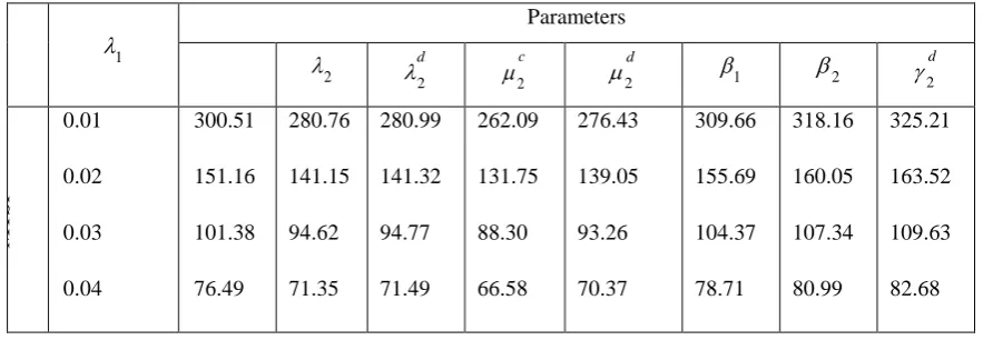
Table 2: Effect of various parameters on MTSF, Availability and Profit with respect to λ1

1



Parameters

2



d

2

 c

2



₂d



1



2

d

2



MT

SF

0.01

0.02

0.03

0.04

300.51

151.16

101.38

76.49

280.76

141.15

94.62

71.35

280.99

141.32

94.77

71.49

262.09

131.75

88.30

66.58

276.43

139.05

93.26

70.37

309.66

155.69

104.37

78.71

318.16

160.05

107.34

80.99

325.21

163.52

109.63

2643 | P a g e

Av

ailab

ilit

y

0.01

0.02

0.03

0.04

0.99841

0.99684

0.99528

0.99373

0.99830

0.99662

0.99495

0.99329

0.99830

0.99662

0.99495

0.99329

0.99818

0.99638

0.99459

0.99282

0.99827

0.99656

0.99487

0.99319

0.99876

0.99752

0.99629

0.99507

0.99850

0.99701

0.99554

0.99408

0.99853

0.99708

0.99564

0.99421

Case-3: When shape parameter η=2

In this case the Weibull distribution reduces to Rayleigh distribution and we get the following:

) exp( 2 )

( _{1 1} 2

1 t t t

z    _, z₂(t)2₂texp(₂t2), z_d2(t)2



₂dtexp(



d₂t2), s₂(t)2₂ctexp(₂ct2),

) exp( 2

)

( _{2 2} 2

2 t t t

s_d 



d 



d , g₁(t)2₁texp(₁t2)

, () 2 exp( )

2

2 2

2 t t t

g    , f_d2(t)2



₂dtexp(



₂dt2) ,

ly. respective

0 , , , , , , , , and 0

t _{1 2 2}d ₂c ₂d _{1 2 2}d 

where         

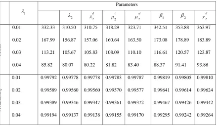
Table 3:Effect of various parameters on MTSF, Availability and Profit with respect to λ1

1



Parameters

2



d

2

 c

2



₂d



1



2

d

2



MT

SF

0.01

0.02

0.03

0.04

332.33

167.99

113.21

85.82

310.50

156.87

105.67

80.07

310.75

157.06

105.83

80.22

318.29

160.64

108.09

81.82

323.71

163.50

110.10

83.40

342.51

173.08

116.61

88.37

353.88

178.89

120.57

91.41

363.97

183.89

123.87

93.86

Av

ailab

ilit

y

0.01

0.02

0.03

0.04

0.99792

0.99589

0.99389

0.99194

0.99778

0.99560

0.99346

0.99137

0.99778

0.99560

0.99347

0.99138

0.99783

0.99570

0.99361

0.99155

0.99787

0.99577

0.99372

0.99170

0.99819

0.99641

0.99467

0.99295

0.99805

0.99614

0.99426

0.99242

0.99810

0.99624

0.99442

0.99264

7.

DISCUSSION AND CONCLUSION

The numerical effect of change in values of different parameters on the reliability and availability is shown in

Tables 1-3. Table 1 gives thevalues of MTSF and availability when the shape parameter of Weibull distribution

η=0.5. Whereas Table 2 and Table 3 gives the values of MTSF and availability,w.r.t. the failure rate of the

2644 | P a g e

exhibit similar results. Both the performance measures declines with increasing values of

1



,

2



, d

2

 , c

2



and d

2



but the trend declines with increasing values of



₁,



₂and₂d.Therefore the numerical results reveal thatunder the stated framework a cold standby system can be made more reliable and available for use by keeping:

a. the failure rate of both units under control b. maximum redundancy times lower

c. repair times of both the units higher and d. faster replacement rate of failed unit.

Acknowledgement:

The authors are very thankful to the reviewers for valuable comments and suggesitions.

REFERENCES

[1] S. K. SrinivasanandM. N. Gopalan, Probabilistic analysis of a 2-unit cold-standby system with a single

repair facility, IEEE Transactions on Reliability, 22(5),1973, 250-254.

[2] K.Murari andV. Goyal, Comparison of two unit cold standby reliability models with three types of

repair facilities, Microelectronics Reliability, 24(1),1984, 35-49.

[3] S. K. Singh andB. Srinivasu, Stochastic analysis of a two unit cold standby system with preparation

time for repair, Microelectronics Reliability, 27(1), 1987, 55-60.

[4] J. Cao andY. Wu, Reliability analysis of a two-unit cold standby system with a replaceable repair

facility, Microelectronics Reliability, 29(2),1989, 145-150.

[5] R. Subramanian and V. Anantharaman, Probabilistic analysis of a three unit cold standby redundant

system with repair, Microelectronics Reliability, 35(6),1995, 1001-1008.

[6] K. M. El-Said andM. S. El-Sherbeny, Stochastic analysis of a unit cold standby system with

two-stage repair and waiting time, Sankhya B, 72(1),2010, 1-10.

[7] R. K. Bhardwaj and S, C. Malik , Asymptotic performance analysis of 2oo3 cold standby system with

constrained repair and arbitrary distributed inspection time, International Journal of Applied

Engineering Research, 6(08), 2011, 1493-1502.

[8] X. Bao and L. Cui, A study on reliability for a two-item cold standby Markov repairable system with

neglected failures, Communications in Statistics-Theory and Methods, 41(21), 2012, 3988-3999.

[9] R. K. Bhardwaj and K. Kaur,Reliability and Profit Analysis of a Redundant System with Possible

Renewal of Standby Subject to Inspection, Int. J. of Stat. &Reliab. Eng, 1(1), 2014, 36–46.

[10] R. K. Bhardwaj and R. Singh, Semi Markov approach for asymptotic performance analysis of a

standby system with server failure, Int. J Comput. Appl, 98(3),2014, 9-14.

[11] R. K. Bhardwaj and R. Singh, Steady state behavior of a cold standby system with server failure and

arbitrary repair, replacement & treatment, International Journal of Applied Engineering Research,

9(24),2014, 26563-26578.

[12] R. K. Bhardwaj, K. Kaur and S. C. Malik, Stochastic Modeling of a System with Maintenance and

Replacement of Standby Subject to Inspection, American J. of Theoretical & Applied Statistics,

2645 | P a g e

[13] R. K. Bhardwaj and R. Singh, An inspection-repair-replacement model of a stochastic standby system

with server failure, Mathematics in Engineering, Science & Aerospace (MESA), 6(2), 2015, 191-203.

[14] R. K. Bhardwaj, K. Kaur and S. C. Malik, Reliability indices of a redundant system with standby

failure and arbitrary distribution for repair and replacement times, International Journal of System

Assurance Engineering and Management, 8(2), 2017, 423-431.

[15] W. L. Smith, Regenerative stochastic processes, Proceedings of the Royal Society of London, Series A.

Mathematical and Physical Sciences, 232(1188), 1955, 6-31.

[16] D. R. Cox, Renewal theory, Methuen and co. Ltd., London, 1962.