Advanced Segmentation Using Echo State Neural Network over Fmri

(1)

Advanced Segmentation Using Echo State Neural Network over

Fmri

M.Kesavi, Dr.D.Haritha [Ph.D

Associate

Professor Dept Of Cse

University College Of

Engineering

Kakinada [Autonomous]

Jjawaharlal Nehru Technological University Kakinada

This research work proposes a new intelligent segmentation technique for

functional Magnetic Resonance Imaging (fMRI). It has been implemented using

an Echostate Neural Network (ESN). Segmentation is an important process that

helps in identifying objects of the image. Existing segmentation methods are not

able to exactly segment the complicated profile of the fMRI accurately.

Segmentation of every pixel in the fMRI correctly helps in proper location of

tumor. The presence of noise and artifacts poses a challenging problem in proper

segmentation. The proposed ESN is an estimation method with energy

minimization. The estimation property helps in better segmentation of the

complicated profile of the fMRI. The performance of the new segmentation

method is found to be better with higher peak signal to noise ratio (PSNR) of 61

when compared to the PSNR of the existing back-propagation algorithm (BPA)

segmentation method which is 57.

Keywords

:

Echo state neural network, Intelligent segmentation, functional magnetic resonance imaging, Back-propagation algorithm, Feature Extraction, Peak signal to noise ratio

1. INTRODUCTION

Medical imaging plays a vital role in the field of bio-medical engineering. Some of the organs of the human body require non-invasive approach to understand the defects such as tumor, cancer in different parts of the body. Study and analysis of brain are done through the images acquired by various modalities like X-ray, Computer Tomography (CT), Positron Emission Tomography (PET), Ultrasound (US), Single Photon Emission Computed Tomography (SPECT) etc. The present day to day study of brain is much preferred through functional magnetic resonance imaging (fMRI). The acquired fMRI image need to be preprocessed, registered and segmented for understanding the defects in the brain by physician. Current tomographic technologies

in medical imaging enable studies of brain function by measuring hemodynamic changes related to changes in neuronal activity. The signal changes observed in functional magnetic resonance imaging (fMRI) are mostly based on blood oxygenation level dependent (BOLD) contrast and are usually close to the noise level. Consequently, statistical methods and signal averaging are frequently used to distinguish signals from noise in the data. In most fMRI setup, images are acquired during alternating task (stimulus) and control (rest) conditions.

(2)

region-based and contour-based approaches. Anatomical knowledge, used appropriately, boost the accuracy and robustness of the segmentation algorithm. MRI segmentation strive toward improving the accuracy, precision and computation speed of t5he segmentation algorithms [10].

Statistical methods are used for determining non-parametric thresholds for fMRI statistical maps by resampling fMRI data sets containing block shaped BOLD responses. The complex dependence structure of fMRI noise precludes parametric statistical methods for finding appropriate thresholds. The non-parametric thresholds are potentially more accurate than those found by parametric methods. Three different transforms have been proposed for the resampling: whitening, Fourier, and wavelet transforms. Resampling methods based on Fourier and wavelet transforms, which employ weak models of the temporal noise characteristic, may produce erroneous thresholds. In contrast, resampling based on a pre-whitening transform, which is driven by an explicit noise model, is robust to the presence of a BOLD response [9].

A commonly used method based on the maximum of the background mode of the histogram, is maximum likelihood (ML) estimation that is available for estimation of the variance of the noise in magnetic resonance (MR) images. This method is evaluated in terms of accuracy and precision using simulated MR data. It is shown that this method outperforms in terms of mean-squared-error [11].

A fully automated, parametric, unsupervised algorithm for tissue classification of noisy MRI images of the brain has been done. This algorithm is used to segment three-dimensional, T1-weighted, simulated and real MR images of the brain into different tissues, under varying noise conditions [12]. Parametric and non-parametric statistical methods are powerful tools in the analysis of fMRI data [7].

Probabilistic approaches to voxel based MR image segmentation identify partial volumetric estimations. Probability distributions for brain tissues is intended to

measurement system [8]. Maximum Posterior Marginal (MPM) minimization and Markov Field [13] were used for contextual segmentation. Functional MRI segmentation using fuzzy clustering technique is proposed for objective determination of tumor volumes as required for treatment monitoring. A combination of knowledge based techniques and unsupervised clustering, segment MRI slices of the brain. Knowledge based technique is essential both in time and accuracy to expand single slice processing into a volume of slices [14].

A method for semiautomatic segmentation of brain structures such as thalamus from MRI images based on the concept of geometric surface flow has been done. The model evolves by incorporating both boundary and region information following the principle of variational analysis. The deformation will stop when an equilibrium state is achieved [15]. Energy minimization algorithm provides a high quality segmentation due to region homogeneity and compactness. The graph algorithm for multiscale segmentation of three dimensional medical data sets has been presented [4].

2. PROBLEM DEFINITION1

The proposed method focuses on a new segmentation approach using energy minimizing echo state neural network. Due to the complicated profiles of the brain, the new method helps in segmenting the profiles by learning the2 different states of the profile of fMRI. Statistical features are calculated from the fMRI. These features are learnt by the training phase of the ESN. The learnt weights are further used for segmentation of the fMRI during the testing phase.

2

3. ECHO

STATE

NEURAL

NETWORK (ESN)

(3)

differential equations. The nodes are interconnected layer-wise or intra-connected among themselves. Each node in the successive layer receives the inner product of synaptic weights with the outputs of the nodes in the previous layer [1]. The inner product is called the activation value.

Dynamic computational models require the ability to store and access the time history of their inputs and outputs. The most common dynamic neural architecture is the time-delay neural network (TDNN) that couples delay lines with a nonlinear static architecture where all the parameters (weights) are adapted with the back propagation algorithm (BPA). Recurrent neural networks (RNNs) implement a different type of embedding that is largely unexplored. RNNs are perhaps the most biologically plausible of the artificial neural network (ANN) models. One of the main practical problems with RNNs is the difficulty to adapt the system weights. Various algorithms, such as back propagation through time and real-time recurrent learning, have been proposed to train RNNs. These algorithms suffer from computational complexity, resulting in slow training, complex performance surfaces, the possibility of instability, and the decay of gradients through the topology and time. The problem of decaying gradients has been addressed with special processing elements (PEs).

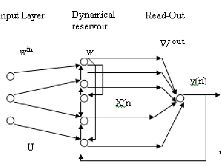
The echo state network, Figure 1, with a concept new topology has been found by [3]. ESNs possess a highly interconnected and recurrent topology of nonlinear PEs that constitutes a “reservoir of rich dynamics” and contain information about the history of input and output patterns. The outputs of this internal PEs (echo states) are fed to a memory less but adaptive readout network (generally linear) that produces the network output. The interesting property of ESN is that only the memory less readout is trained, whereas the recurrent topology has fixed connection weights. This reduces the complexity of RNN training to simple linear regression while preserving a recurrent topology, but obviously places important constraints in the overall architecture that have not yet been fully studied.

The echo state condition is defined in terms of the spectral radius (the largest among the absolute values of the eigenvalues of a matrix, denoted by ( || || ) of the reservoir’s weight matrix (|| W || < 1)). This condition states that the dynamics of the ESN is uniquely controlled by the input, and the effect of the initial states vanishes. The current design of ESN parameters relies on the selection of spectral radius. There are many possible weight matrices with the same spectral radius, and unfortunately they do not all perform at the same level of mean square error (MSE) for functional approximation.

ESN is composed of two parts [5]: a fixed weight (|| W || < 1) recurrent network and a linear readout. The recurrent network is a reservoir of highly interconnected dynamical components, states of which are called echo states. The memory less linear readout is trained to produce the output [6]. Consider the recurrent discrete-time neural network given in Figure 1 with M input units, N internal PEs, and L output units. The value of the input unit at time n is

u (n) = [u1 (n), u2(n), . . . , uM(n)] T

,

The internal units are x(n) = [x1(n), x2(n), .

. . , xN(n)] T

, and

output units are y(n) = [y1(n), y2(n), . . . , yL

(n)]T.

(4)

The connection weights are given

 in an (N x M) weight matrix

back ij back

W



for

connections between the

input and the internal PEs,

 in an N × N matrix

in ij in

W



for connections

between the internal PEs

 in an L × N matrix

out ij out

W



for

connections from PEs to the

output units and

 in an N × L matrix

back ij back

W



for the

connections that project

back from the output to the

internal PEs.

The activation of the internal PEs (echo

state) is updated according to

x(n + 1) = f(Win u(n + 1) + Wx(n) +Wbacky(n)),

(1)

where

f = ( f1, f2, . . . , fN) are the internal

PEs’ activation functions.

All fi’s are hyperbolic tangent

functions _x _x x x

e

 





. The output from the

readout network is computed according to

y(n + 1) = fout(Woutx(n + 1)), .

(2)

where

)

f

,....,

f

,

(f

f

out

L out 2 out 1 out



are the

output unit’s nonlinear functions. The

training and testing procedures are

given in section 5.

4. PROPOSED METHOD FOR

INTELLIGENT SEGMENTATION

(5)

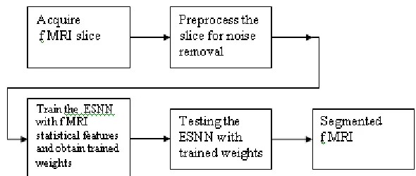
FIGURE 2: Schematic diagram of the Intelligent segmentation

This process is very important for further study of the fMRI slices. The ESN is initialized with random weights. The statistical features obtained from the FMRI are used to train the ESN. The process of training is used to obtain set of trained weights. Testing of ESN is done for fMRI segmentation using the trained weights.

5. IMPLEMENTATION

OF

SEGMENTATION USING ESN

sTraining of ESN to obtain trained weights

Step 1: Find the statistical features of the registered image

Step 2: Fix the target values(labeling) Step 3: Set the no. of inputs, no. of reservoirs , no. of outputs

Step 4: Initialize weight matrices- no. of reservoirs versus no. of inputs, no.of outputs versus no. of reservoirs, no. of reservoirs versus no. of reservoirs Step 5: Initialize temporary matrices.

Step 6: Find values of matrices less than a threshold

Step 7: Apply heuristics by finding eigenvector of updated weight matrices. Step 8: Create network training dynamics and store the final weights.

Implementation of ESN for segmentation of fMRI using the trained weights of

ESN

Step 1: Read the trained weights

Step 2: Input the statistical features of fMRI. Step 3: Process the inputs and fMRI

Step 4: Apply transfer function

Step 5: Find the next state of the ESN. Step 6: Apply threshold and segment the image

6. EXPERIMENTAL SETUP

The fMRI was obtained with standard setup conditions. The magnetic resonance imaging of a subject was performed with a 1.5-T Siemens Magnetom Vision system using a gradient-echo echoplanar (EPI) sequence (TE 76 ms, TR 2.4 s, flip angle 90 , field of view 256 - 256 mm, matrix size 64 * 64, 62 slices, slice thickness 3 mm, gap 1 mm), and a standard head coil. A checkerboard visual stimulus flashing at 8 Hz rate (task condition, 24 s) was alternated with a visual fixation marker on a gray background (control condition, 24 s).

7. RESULTS AND

DISCUSSION

(6)

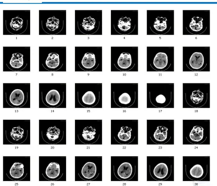
FIGURE 3: fMRI sequences

The image numbered (2) is considered for analyzing the performance of segmentation by ESN algorithm. As the

(7)

(a) Source-1

(b) Source-1 filtered

(c) BPA segmentation

(d) ESN segmentation

FIGURE 4: Segmentation of fMRI – Sequence of outputs

For the comparison of the segmentation performances of the ESN, BPA segmentation is taken as the reference, since BPA is the oldest neural network method used earlier for image segmentation. The segmented image through BPA is shown in Figure 4(c). Similarly the segmented image using ESN is shown in Figure 4(d).

The preprocessing steps in fetal brain

MRI analysis: (a) shows the out-of-plane

view (coronal view) of an original axial

T2wSSFSE scan, (b) is the volumetric

image obtained from iterations of

inter-slice motion correction and robust

super-resolution volume reconstruction, (c)

shows the brain mask obtained through

supervised levelset segmentation and

manual refinement, and (d) is the

reconstructed image, reoriented and

co-registered

to

the

common

atlas

coordinate space after N4 bias field

correction and intensity normalization.

One of the important segmentation performance comparison is PSNR. The PSNR is expressed as

PSNR = 10*log10 (255*255/MSE) ………..….

. (3)

MSE= ∑ (Original image –segmented image)2

where

(8)

FIGURE 5: Comparison performance of ESN and BPA

Figure 5 shows peak signal to noise ratio for different threshold used in both the BPA and ESN algorithms. The PSNR values starts with minimum 57 and goes upto approximately 61. The range of PSNR for the segmented image using BPA is 57 to 58. The PSNR value for the segmented image by ESN ranges from 60 to 61. The maximum PSNR value is obtained in case of ESN

segmentation is for threshold of 0.01 with 60.58. In case of segmentation by BPA, the maximum PSNR is only 57.9 for the threshold of 0.07. By comparison, the maximum PSNR is obtained at lower threshold for the ESN algorithm. The PSNR can be further improved by further modifying the ESN algorithm in terms of number of nodes I the hidden layer.

(9)

Frequency distribution of subjects

contributed to atlas construction at each

gestational age point in weeks. The

number of subjects used in atlas

construction at lower GAs was, on

average, smaller than the numbers at

higher GAs, which was acceptable as the

fetal brain has less features and

variability at lower GAs compared to

higher GAs.

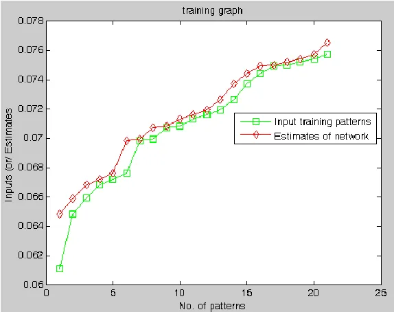
The Figure 6 shows the ESN estimation and the corresponding input patterns. The estimate is based on the number of reservoirs used during the training process.

8. CONCLUSION

The fMRI segmentation has been done with a recurrent ESN that stores the different states of fMRI. The PSNR value for this method is 60.6867. whereas, the PSNR value for the segmentation done by back-propagation algorithm is 55.67. The work can be further extended by incorporating modifications of internal states in ESN and fine tuning the noise filtering methods.

9. REFERENCES

[1] Rumelhart D.E., Hinton G.E., and William R.J; Learning internal representations by error propagation, in Rumelhart, D.E., and McClelland, J.L.; Parallel distribution processing: Explorations in the microstructure of cognition; 1986.

[2] Lippmann.R.P,; An Introduction to computing with neural nets, IEEE Transactions on ASSP Mag.,.35,4-22, 1987. [3] Jaeger, H.; The echo state approach to analyzing and training recurrent neural networks; (Tech. Rep. No. 148). Bremen: German National Research Center for Information Technology, 2001.

[5] Jaeger, H;. Short term memory in echo state networks; (Tech. Rep. No. 152) Bremen: German National Research Center for Information Technology. 2002.

[6] Jaeger, H.; Tutorial on training recurrent neural networks, covering BPPT, RTRL,EKF and the “echo state network” approach

(Tech. Rep. No. 159).; Bremen: German National Research Center for Information Technology, 2002.

[7] Sinisa Pajevica and Peter J. Basser, Parametric and non-parametric statistical analysis of DT-MRI data, Journal of Magnetic Resonance,1–14, 2003.

[8] Thacker N. A., D. C. Williamson, M. Pokric; Voxel Based Analysis of Tissue Volume MRI Data;20th July 2003

[9].Ola Friman and Carl-Fredrik Westin; Resampling fMRI time series; NeuroImage 25, 2005

[10].Alan Wee-Chung Liew and Hong Yan; Current Methods in the Automatic Tissue Segmentation of 3D Magnetic Resonance Brain Images; Current Medical Imaging Reviews, 2006.

[11] D. Poot, J. Sijbers,3A. J. den Dekker, R. Bos;Estimation of the noise variance from the background histogram mode of an mr image, Proceedings of SPS-DARTS,2006

[12] Hayit Greenspan, Amit Ruf, and Jacob Goldberger, Constrained Gaussian Mixture Model Framework for Automatic Segmentation of MR Brain Images, IEEE Transactions On Medical Imaging, 25 (9), SEPTEMBER 2006

[13] Abdelouahab Moussaoui, Nabila Ferahta, and Victor Chen; A New Hybrid RMN Image Segmentation Algorith.; Transactions On Engineering, Computing And Technology, 12 ,2006

[14]. Ruth Heller, Damian Stanley, Daniel Yekutieli, Nava Rubin, and Yoav Benjamini; Cluster-based analysis of FMRI data; NeuroImage 599–608, 2006