Effects of Surface Topographies on Heat and Fluid Flows

(1)

Scholarship@Western

Electronic Thesis and Dissertation Repository

1-10-2014 12:00 AM

Effects of Surface Topographies on Heat and Fluid Flows

Hadi Vafadar Moradi

The University of Western Ontario

Supervisor

Dr. Jerzy Maciej Floryan

The University of Western Ontario

Graduate Program in Mechanical and Materials Engineering

A thesis submitted in partial fulfillment of the requirements for the degree in Doctor of Philosophy

Follow this and additional works at: https://ir.lib.uwo.ca/etd

Part of the Mechanical Engineering Commons

Recommended Citation Recommended Citation

Vafadar Moradi, Hadi, "Effects of Surface Topographies on Heat and Fluid Flows" (2014). Electronic Thesis and Dissertation Repository. 1878.

https://ir.lib.uwo.ca/etd/1878

This Dissertation/Thesis is brought to you for free and open access by Scholarship@Western. It has been accepted for inclusion in Electronic Thesis and Dissertation Repository by an authorized administrator of

(2)

(Thesis format: Monograph)

by

Hadi Vafadar Moradi

Graduate Program in Engineering Science Department of Mechanical and Materials Engineering

A thesis submitted in partial fulfillment of the requirements for the degree of

Doctor of Philosophy

The School of Graduate and Postdoctoral Studies The University of Western Ontario

London, Ontario, Canada

(3)

ii

Abstract

Responses of annular and planar flows to the introduction of grooves on the bounding surfaces have been analyzed. The required spectral algorithms based on Fourier and Chebyshev expansions have been developed. The difficulties associated with the irregularities of the physical domain have been overcome using either the immersed boundary conditions (IBC) concept or the domain transformation method (DT).

Steady flows in annuli bounded by walls with longitudinal grooves have been studied. Analysis of pressure losses showed that the groove-induced changes can be represented as a superposition of a pressure drop due to a change in the average position of the bounding cylinders and a pressure drop due to the flow modulations induced by the shape of the grooves. The former effect can be evaluated analytically while the latter requires explicit computations. It has been shown that the reduced-order model is an effective tool for extraction of features of the groove geometry that lead to flow modulations relevant to drag generation. It has been shown that the presence of the longitudinal grooves may lead to a reduction of the pressure loss in spite of an increase of the wetted surface area. The form of the optimal grooves from the point of view of the maximization of the drag reduction has been determined.

When mixing augmentation is not available, heat can be transported across micro-channels by conduction only. A method to increase this heat flow has been proposed. The method relies on the use of grooves parallel to the flow direction. It has been shown that it is possible to find grooves that can increase the heat flow and, at the same time, can decrease the pressure losses. The optimal groove shape that maximizes the overall system performance has been determined. Since it has been assumed that the flow must be laminar, it is of interest to determine the maximum Reynolds number for which this assumption remains valid.

(4)

iii

numbers < ≈ 4.22 and flow destabilization for larger . The stabilizing/destabilizing effects increase with the groove amplitude. Variations of the critical Reynolds number over the whole range of groove wave numbers and groove amplitudes of interest have been determined. Special attention has been paid to the effects of long wavelength, drag reducing grooves. It has been shown that such grooves lead to a small increase of the critical Reynolds number compared with the smooth channel.

Keywords

(5)

iv

Co-Authorship Statement

(6)

v

To my wife and my parents

(7)

vi

Acknowledgments

It is a pleasure to thank the many people who made this thesis possible. It is difficult to overstate my gratitude to my Ph.D. supervisor, Dr. Jerzy Maciej Floryan. I will remain indebted to Prof. Floryan for his precious time, patience, enthusiasm, inspiration, and his great efforts to explain things clearly and simply. The completion of this dissertation would not have been possible without his incomparable assistance and invaluable guidance.

I would like to extend my sincerest thanks to the member of my advisory committee, Dr. A. G. Straatman, for his valuable suggestions and encouragement.

I would also like to thank all of my colleagues (past and present), Dr. Syed Zahid Husain, Dr. Mohammad Zakir Hossain, Dr. Alireza Mohammadi, Mohammad Fazel Bakhsheshi, David César Del Rey Fernandez, Ali Asgarian for their friendship, cooperation and helping attitude. I am particularly grateful to Alireza not only for the insightful scientific discussions I had with him that have been tremendously helpful for me in achieving my research objectives but also because of friendship, courage, motivation, and support I have received from him.

Words are not enough to express my gratitude towards my wife, Shima Ahmadi. Without her unconditional love, encouragement, tremendous patience and understanding, I would not have been able to accomplish my goals.

(8)

vii

List of Figures

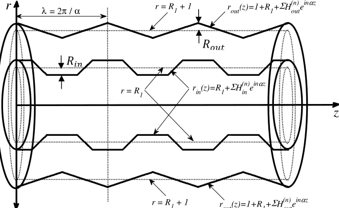
Figure 2-1: Sketch of the flow geometry - axisymmetric annulus with transverse ribs of arbitrary cross-section. ...17

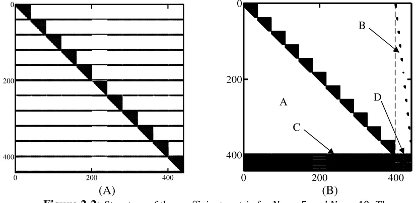
Figure 2-2: Structure of the coefficient matrix for = 5 and = 40. The nonzero

elements are marked in black. The total number of elements, the number of nonzero elements and the sparsity (ratio of the number of the zero elements to the total number of the elements) for this matrix are 440= 193600, 27780 and 0.86, respectively. Figure 2-2A - the structure of the coefficient matrix before the re-arrangement, Figure 2-2B - the structure of the coefficient matrix after the re-arrangement (see Section 2.2.5 for a discussion). ...31

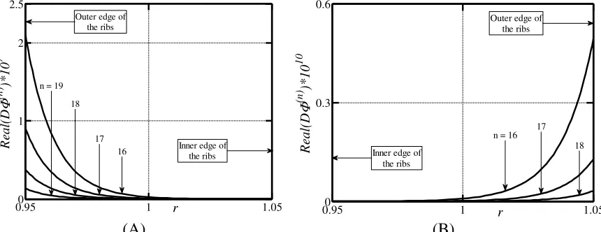
Figure 2-3: Distribution of the real part of as a function of r for higher Fourier modes

> 15 for ribs placed either at the inner cylinder (Figure 2-3A) or at the outer cylinder (Figure 2-3B). The geometry of the ribs' is given by Eq. (2.2.52) with the ribs' wave number

= 5, the ribs' amplitude S = 0.05 and the average radius on the inner cylinder = 1. Computations have been carried out for the flow Reynolds number Re = 50 using = 20

Fourier modes and = 70 Chebyshev polynomials. ...33

Figure 2-4: Variations of the Chebyshev norm defined by Eq. (2.2.53) as a function of the Fourier mode number n for the model geometry described by Eq. (2.2.52) with the ribs' wave number = 2 for selected values of the ribs' amplitude S (Figure 2-4A) and with the ribs' amplitude S = 0.04 for selected values of the ribs' wave numbers (Figure

2-4B). Calculations have been carried out for the flow Reynolds number Re = 50 and the

average radius of the inner cylinder = 1.5 using = 20 Fourier modes and = 70 Chebyshev polynomials. ...34

Figure 2-5: Variations of the Chebyshev norm defined by Eq. (2.2.53) as a function of the Fourier mode number n for the model geometry described by Eq. (2.2.52) with the ribs' amplitude = 0.04, the ribs' wave number = 2 and the average radius of the inner cylinder = 1.5 for selected values of the flow Reynolds number Re. Calculations

(13)

xii

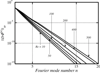
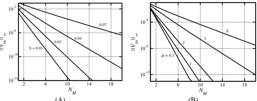
Figure 2-6: Variations of the norm ‖"_#‖_$ defined by Eq. (2.2.54) as a function of the number of Fourier modes used in the computations for the model problem described by Eq. (2.2.52) with the ribs' wave number = 5 for selected values of the ribs' amplitude S

(Figure 2-6A) and with the ribs' amplitude S = 0.04 for selected values of the ribs' wave

number (Figure 2-6B). Calculations have been carried out for the flow Reynolds number

Re = 50 and the average radius of the inner cylinder = 1 using = 70 Chebyshev

polynomials. ...36

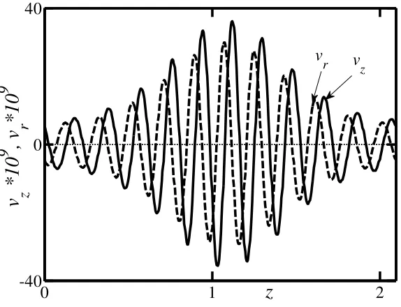
Figure 2-7: Distributions of the velocity components %_& and % evaluated along the inner cylinder for the model geometry described by Eq. (2.2.52) with the ribs' wave number = 3, the ribs' amplitude S = 0.05 and the average radius of the inner cylinder = 1. Calculations

have been carried out for the flow Reynolds number Re = 50 using = 10 Fourier modes

and = 40 Chebyshev polynomials. ...37

Figure 2-8: Fourier spectra of the velocity components %_& and % (Figure 2-8A) and of the

stream function derivatives () (*⁄ and () (,⁄ (Figure 2-8B) evaluated at the surface of the inner cylinder. Other conditions as in Figure 2-7. ...38

Figure 2-9: Fourier spectra of the axial velocity component %_& evaluated at the surface of the inner cylinder for ribs with the wavelength - = 2. 3⁄ . Other conditions as in Figure 2-7. Solution have been obtained with = 3 and = 10 in case A, = 1.5 and = 20 in case B, and = 1 and = 30 in case C. ...39

Figure 2-10: Variations of the norms ‖"_#‖_$ and ‖"_/0‖_$ defined by Eq. (2.2.54) as a

function of the radius of the inner cylinder . The former one corresponds to an annulus with geometry described by Eq. (2.2.52) with the ribs' wave number = 4 and the ribs' amplitude S = 0.06. The latter one corresponds to the same ribs but placed at the outer

cylinder. Computations were carried out for the flow Reynolds number Re = 10 using = 20 Fourier modes and = 70 Chebyshev polynomials. ...39

Figure 2-11: Variation of the norm ‖"_#‖_$ defined by Eq. (2.2.54) as a function of the flow Reynolds number Re for an annulus with geometry defined by Eq. (2.2.52) with the ribs'

(14)

xiii

= 1 determined using different number of Fourier modes and = 70 Chebyshev

polynomials. ...40

Figure 2-12: Variations of the norm ‖"_#‖_$ defined by Eq. (2.2.54) as a function of the ribs'

amplitude S for selected values of the ribs' wave numbers (Figure 2-12A) and as a function

of the ribs' wave number for selected values of the ribs' amplitude S (Figure 2-12B) for the model configuration described by Eq. (2.2.52). Calculations have been carried out for the flow Reynolds number Re = 50 and the average radius of the inner cylinder = 1 using = 20 (solid lines) and = 15 (dashed line) Fourier modes, and = 70 Chebyshev polynomials. ...41

Figure 2-13: Variations of the additional pressure loss generated by the ribs with geometry defined by Eq. (2.2.52) as a function of the rib’s amplitude S and the ribs' wave number for the flow Reynolds number Re = 10 and the average radius of the inner cylinder = 1. 42

Figure 2-14: Variations of the additional pressure loss generated by the ribs with geometry given by Eq. (2.2.52) as a function of the flow Reynolds number Re and the average radius

of the inner cylinder for ribs with the wave number = 2 and the amplitude S = 0.04. ...42

Figure 2-15: Streamlines of a flow in an annulus with geometry defined by Eq. (2.2.55) for the flow Reynolds number Re = 10. ...43

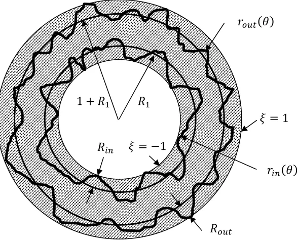
Figure 2-16: Sketch of the flow geometry - annulus with axial ribs of arbitrary form. Shaded area represents computational domain. ...44

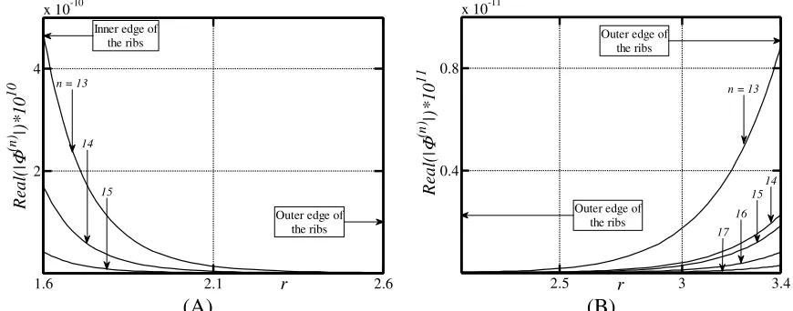
Figure 2-17: Distribution of the real part of as a function of r for higher Fourier

modes > 13 in the region close to the surfaces of the inner (Figure 2-17A) and outer (Figure 2-17B) cylinders. The ribs' geometry is given by Eq. (2.3.37) with the inner and outer amplitudes _# = 0.4 and _/0 = 0.4, respectively, and the average radius on the inner cylinder = 2. Computations have been carried out using = 20 Fourier modes and

= 70 Chebyshev polynomials. ...54

(15)

xiv

ribs' amplitude _#. Calculations have been carried out for the smooth outer cylinder

/0 = 0 and the average radius of the inner cylinder = 2 using = 20 Fourier modes

and = 70 Chebyshev polynomials. ...55

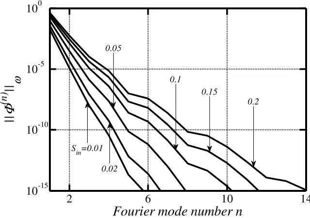
Figure 2-19: Variations of the norm ‖"_#‖_$ defined by Eq. (2.3.38) as a function of the number of Fourier modes used in the computations for the model problem described by Eq. (2.3.37) for selected values of the inner ribs' amplitude _#. Calculations have been carried out for the smooth outer cylinder _/0 = 0 and the average radius of the inner cylinder = 1 using = 70 Chebyshev polynomials. ...56

Figure 2-20: Variations of the norm ‖"_#‖_$ defined by Eq. (2.3.38) as a function of the ribs' inner amplitude _# for the model configuration described by Eq. (2.3.37). Calculations have been carried out for the smooth outer cylinder _/0 = 0 and the average radius of the inner cylinder = 1 using = 70 Chebyshev polynomials and selected number of the Fourier modes . ...56

Figure 2-21: Distributions of the axial velocity component %_& evaluated along the inner and

outer cylinders for the model geometry described by Eq. (2.3.37) with the ribs' inner and outer amplitudes _/0 = 0.05 and _/0 = 0.1, respectively, and 1 replaced by 31. Calculations have been carried out for the average radius of the inner cylinder = 1 using

= 20 Fourier modes and = 70 Chebyshev polynomials. ...57

Figure 2-22: Fourier spectra of the axial velocity component %_& evaluated along the inner and outer cylinders for the model geometry described by Eq. (2.3.37). Other conditions as in Figure 2-21. ...58

Figure 2-23: Variations of the norms ‖"_#‖_$ and ‖"_/0‖_$ defined by Eq. (2.3.38) as a

(16)

xv

Figure 2-24: Variations of the additional pressure loss 2 (3⁄(, associated with the presence of the ribs at the inner cylinder while the outer cylinder is kept smooth _/0 = 0 as a function of the ribs' amplitude _# and the average radius of the inner cylinder . The ribs' geometry is defined by Eq. (2.3.37). Computations were carried out using = 20 Fourier modes and = 70 Chebyshev polynomials. ...59

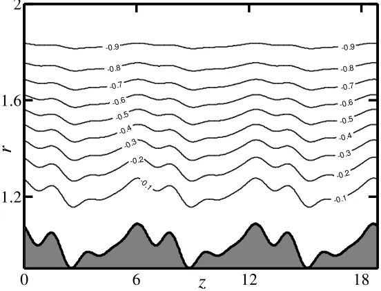
Figure 2-25: Velocity contours for the model problem defined by Eq. (2.3.39). ...60

Figure 3-1: Sketch of the flow geometry - annulus with longitudinal grooves with an arbitrary geometry. ...63

Figure 3-2: Variations of the error of the asymptotic approximation for → ∞. Solid lines

correspond to grooves placed at the inner cylinder (Eq. 3-6) with M = 8 and _# = 0.15 and dashed lines correspond to the same grooves placed at the outer cylinder (see Eq. B-1). ...68

Figure 3-3: Variations of the geometric correction factors _#,7 and _/0,7 as functions of for the groove geometry described by Eq. (3.4.3) with _89,# = _89,/0 = : = 0 with the same grooves placed either at the inner cylinder (solid lines, _# = 0.1, _/0 = 0) or at the outer cylinder (dashed lines, _# = 0, _/0 = 0.1). ...76

Figure 3-4: Sketch of the test configuration used to demonstrate the effect of the average position _89,# of the grooves. Four grooves (M = 4) with the shape defined by Eq. (3.4.3)

with _# = 0.3, _/0 = 0, _89,/0 = 0 are placed at three different average locations: Case A – _89,#= 0.3; Case B – _89,#= 0; Case C – _89,#= −0.3. See text for details. ...78

Figure 3-5: Variations of the normalized modification friction factor ;⁄;_< as a function of the groove amplitude _# for = 1. Four grooves (M = 4) are placed at the inner cylinder with their geometry described by Eq. (3.4.3) with _89,/0 = _/0 = 0 and _89,# = 0.05, 0, −0.05 in Cases A, B, C, respectively. ...78

Figure 3-6: Shapes of the grooves used in this study: A- rectangular groove, B- trapezoidal

(17)

xvi

Figure 3-7: Variations of the normalized modification friction factor ;⁄;_< as a function of the number of Fourier modes _A used to describe the groove geometry. Four grooves (M = 4)

with shapes described in Figure 3-6 and the same amplitude _#= 0.1 are placed at the inner cylinder with the average radius = 1 in such a way that mode zero of their Fourier expansion is zero. For grooves A: B = C = . @⁄ ; for grooves B: B = C = . 3@⁄ , D =

2. 3@⁄ . ...81

Figure 3-8: Variation of the normalized modification friction factor ;⁄;_< as a function of

for the geometry described by (3.4.3) with _89,/0 = _/0 = 0 and @ = 2, 5 and 10. Solid (dashed) lines correspond to the same grooves placed only on the inner (outer) cylinder with

# = 0.3, /0 = 0 ( /0 = 0.3, # = 0 ). ...82

Figure 3-9: Variations of the normalized modification friction factor ;⁄;_< as a function of the groove amplitudes _# and _/0 and the radius of the inner cylinder for the geometry described by Eq. (3.4.3) with _89,/0 = _89,# = 0. Results for M = 2, 4, 10, 15 grooves are displayed in Figure 3-9A, B, C, D, respectively. Solid (dashed) lines correspond to grooves placed only at the inner (outer) cylinder. ...83

Figure 3-10: Variations of the normalized modification friction factor ;⁄;_< induced by the

grooves placed at the inner cylinder with the shape defined by Eq. (3.4.3) with _89,/0 =

89,# = /0 = 0 and M = 4, as a function of the amplitude # (solid lines) and as a

function of the wave number = @/ (dashed lines). ...84

Figure 3-11: Variations of the critical groove wave number ₇ as a function of the number of grooves M for an annulus with geometry described by Eq. (3.4.3) with _89,/0 = _89,# =

0. Solid (dashed) line corresponds to the grooves placed only at the inner (outer) cylinder with _# = 0.1 and 0.8, _/0 = 0 ( _# = 0, _/0 = 0.1 and 0.8). ...85

Figure 3-12: Variations of the normalized modification friction factor ;⁄;_< as a function of the groove phase difference : and the radius of the inner cylinder for the grooves described by Eq. (3.4.3) with _#= _/0 = 0.3 and _89,/0 = _89,# = 0. Results for M = 5,

(18)

xvii

Figure 3-13: Distribution of the axial component of shear stress acting on the fluid at the

inner (Figure 3-13A) and outer (Figure 3-13B) cylinders for grooves with the geometry defined by Eq. (3.4.3) with _# = 0.3, _/0 = 0, = 5, and _89,/0 = _89,#= 0. Dashed lines provide reference values for the smooth cylinders. ...87

Figure 3-14: Distribution of the axial velocity component in an annulus with the geometry defined by Eq. (3.4.3) with _# = 0.3, = 5, _89,/0 = _89,#= _/0 = 0 and M = 5

(Figure 3-14A) and M = 15 (Figure 3-14B). ...87

Figure 3-15: Distribution of the axial velocity component in an annulus with the geometry defined by Eq. (3.4.3) with _# = _/0 = 0.3, = 5, _89,/0 = _89,#= 0, M = 5, and :

= 0 (Figure 3-15A) and : = . (Figure 3-15B). ...88

Figure 3-16: Variations of the normalized modification friction factor ;⁄;_< as a function of the number of Fourier modes used for description of the optimal shape of the equal-depth grooves placed at the inner cylinder. ...91

Figure 3-17: Evolution of the optimal shape of M = 2, 10 equal-depth grooves placed at the

inner cylinder as a function of the wall curvature . Solid, dashed and dotted lines correspond to the depth of the grooves _#,# = _#,/= S = 0.2, 0.5, 0.8, respectively. All these

lines overlap for = ∞. The other values of shown correspond to values close to those that cause a change from drag reduction to a drag increase (see Figure 3-11). Thick lines describe the universal shape, i.e. trapezoid with B = C = -/6 and D = G = -/3 (see text for details). ...92

Figure 3-18: Variations of the normalized modification friction factor ;⁄;_< for M = 2 equal-depth optimal grooves (Figure 3-18A) and M = 10 similar grooves (Figure 3-18B) placed at

the inner cylinder (solid lines). Modification friction factors for the same grooves approximated using the universal trapezoid are marked using dashed lines. See text for details. ...93

Figure 3-19: Variations of the normalized modification friction factor ;⁄;_< as a function of

the wall curvature and the groove amplitude _#,# = _#,/= S for M = 2 universal

(19)

xviii

at the inner cylinder (see text for discussion). Dashed lines are for the sinusoidal grooves defined by Eq. (3.4.3) with _89,/0= _89,#= 0. ...94

Figure 3-20: Optimal shapes of the equal-depth grooves placed at both cylinders. H1 is defined as IJ_/01 − 1 − L ⁄ _/0,#, IJ_#1 − L ⁄ _#,#. Figure 3-20A displays results for

M = 2 grooves; the solid lines are for = 3, _#,/ = _#,# = _/0,/ = _/0,# = 0.2, the

dotted lines are for = 5, _#,/ = _#,# = _/0,/ = _/0,# = 0.4, and the dash lines are for

= 10, #,/ = #,# = /0,/ = /0,# = 0.4. Figure 3-20B displays results for M = 10

grooves; the solid lines are for = 8, _#,/ = _#,# = _/0,/= _/0,#= 0.2, and the dashed lines are for = 10 and _#,/ = _#,# = _/0,/ = _/0,# = 0.4. ...95

Figure 3-21: Variations of the normalized modification friction factor ;⁄;_< as a function of

the wall curvature and the groove amplitude _#,# = _#,/ = _/0,# = _/0,/= S for M = 2 universal equal-depth trapezoidal grooves (Figure 3-21A) and M = 10 similar grooves

(Figure 3-21B) placed at both cylinders (see text for discussion). Dashed lines are for the sinusoidal grooves defined by Eq. (3.4.3) with _89,/0 = _89,# = 0. The reader should note that the universal trapezoid does not offer a good approximation for the optimal grooves under conditions close to transition between the drag increasing and the drag decreasing geometries. ...96

Figure 3-22: Variations of the normalized modification friction factor ;⁄;_< as a function of the depth of the grooves, i.e. _/0,/, for the unequal-depth grooves. The grooves are placed at the outer cylinder and have the same maximum height set at _/0,# = 0.5. Solid and dashed lines correspond to the use of @ = 2 and @ = 10 grooves, respectively. The dotted (@ = 2) and dashed-dotted (@ = 10) lines identify the depth of the grooves that leads to the maximum drag reduction. ...97

Figure 3-23: Evolution of the optimal shape of the unequal-depth grooves placed at the outer

cylinder as a function of the depth of the groove _/0,/. The height of the groove is set at

/0,# = 0.5. The results presented in Figure 3-23A are for M = 2, = 1, and in Figure 3-23B for M = 10, = 20. Dashed lines illustrate shapes corresponding to the optimal

(20)

xix

Figure 3-24: Shapes of the unequal-depth optimal grooves corresponding to the optimal

depth, i.e. the optimal geometry, for grooves placed at the outer cylinder for selected values of the wall curvature . H1 is defined as IJ_/01 − J_/0_N#L IJ⁄ _/0_NO− J_/0_N#L. The height of the groove is set at _/0,# = 0.5. Figure 3-24A-B present results for M = 2 and

M = 10, respectively. The same shapes, but normalized with the width at half height P_QRS

are presented in Figure 3-24C-D. The universal shape has the form of a Gaussian function defined by T = 2UV.OW and is illustrated using solid lines.. ...98

Figure 3-25: Variations of the normalized modification friction factor (Figure 3-25A), the optimal depth (Figure 3-25B) and the half width of the optimal groove (Figure 3-25C) as a function of the wall curvature for an annulus with the smooth inner cylinder and the optimal geometry of the outer cylinder. The maximum heights of the grooves are set as

/0,# = 0.8 (dashed-dotted lines), /0,# = 0.5 (solid lines) and /0,# = 0.2 (dashed lines).

Dotted lines correspond to the asymptotic solution, i.e. → ∞.. ...100

Figure 3-26: Variations of the normalized modification friction factor (Figure 3-26A), the

optimal depth (Figure 3-26B) and the half width of the optimal groove (Figure 3-26C) as a

function of the wall curvature for an annulus with the optimal geometries of the inner and outer cylinders. The maximum heights of the grooves at the inner and outer cylinders are the same and set at the level of _/0,# = 0.4 (dashed lines) and _/0,# = 0.2 (solid lines). Dotted lines correspond to the asymptotic solution, i.e. → ∞. ...101

Figure 4-1: Sketch of the heat transfer system. ...104

Figure 4-2: Variation of X X⁄ _< as a function of the groove amplitude _Y and the wave

number for the geometry described by Eq. (4.4.1). Dashed lines identify asymptotic values for → 0.. ...113

Figure 4-3: Temperature distribution inside the channel for the grooves described by Eq.

(4.4.1) with the amplitude _Y = 2 and the wave number = 0.5 (Figure 4-3A) and = 30

(Figure 4-3B). ...114

Figure 4-4: Temperature profiles at Z = -_O⁄2 for the grooves described by Eq. ( 4.4.1) with

(21)

xx

Figure 4-5: Distributions of the local heat flux at the lower (Figure 4-5A) and upper (Figure 4-5B) walls for grooves described by Eq. (4.4.1) with the amplitude _Y = 1. ...115

Figure 4-6: Variations of the wetted surface area [ [⁄ _< (see Eq. (4.3.13)) as a function of the

groove amplitude _Y and the wave number for the groove geometry described by Eq. (4.4.1). ...116

Figure 4-7: Variation of ; ;⁄ _< as a function of the groove amplitude _Y and the wave number for the geometry described by Eq. (4.4.1). Dashed lines identify asymptotic values for

→

0. ...117

Figure 4-8: Distribution of the w - velocity component for grooves described by Eq. (4.4.1)

with amplitude _Y = 2 and the wave numbers = 0.5 (Figure 4-8A) and = 5 (Figure 4-8B). ...117

Figure 4-9: Distribution of the z-component of shear acting at the lower (Figure 4-9A) and upper (Figure 4-9B) walls for grooves described by Eq. (4.4.1) with amplitude _Y = 1. ...118

Figure 4-10: Variations of the ; ;⁄ _< and X X⁄ _< for a channel with geometry described by Eq.

(4.4.1) as a function of the groove wave number .. ...119

Figure 4-11: Variations of the thermal enhancement factor Ω for a channel with geometry described by Eq. (4.4.1) as a function of the groove wave number . ...121

Figure 4-12: Variations of the normalized friction factor ; ;⁄ _< and the thermal enhancement

factor Ω for the equal-depth grooves with amplitude _Y = 1 as a function of the number of Fourier modes _A used in the description of the groove geometry. ...123

Figure 4-13: The optimal shapes of the equal-depth grooves. Solid line identifies a groove with _Y = 0.4 and = 0.1, whilst dotted line is for _Y = 1.6 and = 1. The y-coordinate is

scaled using the groove depth. Thick line illustrates the best-fitted trapezoid characterized by

B = C = - 11⁄ and D = G = 4.5- 11⁄ . ...124

Figure 4-14: Velocity isolines for the equal-depth optimal grooves (thick lines) and for the

(22)

xxi

Distributions of the shear stress acting on the fluid at the lower wall for the same grooves are shown in Figure 4-14B. Solid, dashed and dotted lines in Figure 4-14

Figure 4-14B correspond to the optimal groove, the sinusoidal groove and the reference

smooth wall. The corresponding total shear forces are -1.8173, -1.8878 and −2. ...125

Figure 4-15: Variations of the normalized heat transfer per unit length X X⁄ _< (Figure 4-15A),

the normalized friction factor ; ;⁄ _< (Figure 4-15B) and the thermal enhancement factor Ω

(Figure 4-15C) as a function of the groove wave number and the groove depth _Y for a channel with the lower wall fitted with the equal-depth grooves approximated by a trapezoid with B = C = - 11⁄ , D = G = 4.5- 11⁄ and a smooth upper wall. Dashed lines identify results for the simple sinusoidal grooves. ...126

Figure 4-16: Variations of the wetted surface area [ [⁄ _< (see Eq.(4.3.13)) as a function of

the groove wave number for the same grooves as used in Figure 4-15. Dashed lines identify results for the simple sinusoidal grooves...127

Figure 4-17: Variations of the thermal enhancement factor as a function of the groove wave

number for the equal-depth grooves located on the lower wall. Solid and dashed lines correspond to grooves with the optimal and trapezoidal shapes, respectively. ...127

Figure 4-18: The optimal shapes for the equal depth grooves placed on both walls. Solid line

identifies _Y = _] = 0.2 and = 0.1, whilst dotted line is for _Y = _] = 0.5 and = 1 . Thick lines illustrate the best-fitted trapezoids with B = C = 1.25- 11⁄ and D = G =

4.25- 11⁄ . ...128

Figure 4-19: Variations of the thermal enhancement factor Ω as a function of the groove

wave number and the groove depth L for a channel with the lower and upper walls fitted with the equal-depth grooves approximated by a trapezoid with B = C = 1.25- 11⁄ and

(23)

xxii

Figure 4-20: Variations of the thermal enhancement factor Ω for a channel with the smooth upper wall and the optimal grooves with height _Y,NO = 1 placed at the lower wall as a function of the depth of the grooves _Y,N#. ...130

Figure 4-21: Evolution of the shape of the optimal, unequal-depth grooves with height Y,NO = 1 placed on the lower wall as a function of the groove depth Y,N#. Results for = 0.1, 0.5, 1 are displayed in Figure 4-21A, B and C, respectively. Dashed lines identify

shapes corresponding to the optimal depth. ...131

Figure 4-22: Shapes of the unequal-depth grooves with height _Y,NO corresponding to the

optimal depth placed at the lower wall. The y-coordinate is scaled using the groove

peak-to-bottom distance T^_YZ = _T_YZ − _Y,N#` a c _Y,NO− _Y,N#b− 1. Solid, dashed, dash-dotted, and dotted lines correspond to = 0.1, 0.5, 0.8, 1.0, respectively. ...132

Figure 4-23: Shapes of the grooves displayed in Figure 4-22 scaled in the x-direction with the groove width at half height P_QRS (Figure 4-23A). Solid, dashed, dash-dotted, and dotted

lines correspond to = 0.1, 0.5, 0.8, 1.0, respectively. Thick dashed line identifies the universal shape T^Z̅ = −2Z3−3.5Z̅. Variations of the optimal depth _/e and the corresponding width at half height P_QRS as a function of the groove wave number

α

are displayed in Figure 4-23B. ...132

Figure 4-24: Variations of the thermal enhancement factor Ω for the optimal geometry with grooves placed on only one wall. ...133

Figure 4-25: Variations of the thermal enhancement factor Ω (Figure 4-25A) and the

corresponding optimal depth _/e and the width at half height P_QRS (Figure 4-25B) as a

function of the groove wave number for the optimal geometry with grooves placed on both walls and moved by half wavelength with respect to each other. ...133

Figure 5-1: Sketch of the flow system problem. ...137

Figure 5-2: Variations of the error G3 GZ⁄ ₉ of the small wave number approximation of

the stationary state (see Eq. (5.2.23)) and variations of the pressure gradient correction

(24)

xxiii

show the pressure-gradient asymptote for → 0 and the lower bound for the pressure gradient for → ∞. ...142

Figure 5-3: Variations of the pressure gradient correction 2 G3⁄GZ as a function of the groove wave number and the groove height _Y for groove geometry described by Eq. (5.2.21). ...142

Figure 5-4: Distributions of the streamwise velocity f_g in the middle of the groove with

geometry described by Eq. (5.2.21) with _Y = 0.05. ...143

Figure 5-5: Variations of the Chebyshev norm ΦT (see Eq. (5.3.14)) as a function of the Fourier mode number for the groove geometry described by Eq. (5.2.21) with

Y = 0.05, for flow Reynolds number 2 = 6500 and disturbance wave numbers i = 1.02, j = 0. ...149

Figure 5-6: Variations of the growth rate k_#× 10V of disturbances with the wave numbers

i = 1.02 and j = 0 as a function of the number of Fourier modes used in the numerical solution of the stability problem for flow with the Reynolds number Re = 6500 in the

grooved channel with the groove geometry described by Eq. ( 5.2.21) with _Y = 0.05.. ...150

Figure 5-7: Variation of the growth rate k_# × 10V of disturbances with the wave numbers

i = 1.02 and j = 0 as a function of the groove amplitude _Yfor the groove geometry described by Eq. ( 5.2.21) for flow with the Reynolds number 2 = 6500.. ...152

Figure 5-8: Variations of the critical Reynolds number of disturbances with the wave vector

m = i, j of constant magnitude as a function of its inclination angle

θ

for the groove geometry described by Eq. ( 5.2.21) with the amplitude _Y = 0.05. Solid lines correspond to

|m| = 1.02 and dotted lines to|m| =1.0.. ...153

(25)

xxiv

Figure 5-10: Eigenfunctions n₀T, = 0, 1, 2, describing two-dimensional travelling

wave disturbances with the wave number i =1.02 in a channel with grooves whose geometry is described by Eq. ( 5.2.21) with _Y = 0.05. Results displayed in Figs. 5-10A, B, C, and D correspond to the onset conditions for the groove wave numbers =10, 4.22, 1.0, and 0.2, i.e. 2₇ = 5028.5, 5773.5, 5886, and 6227.5, respectively. The normalization condition

oBZp∈I<,Lrn0<Tr = 1 has been used for the presentation purposes. Solid and dash lines

identify the real and imaginary parts. Thin dashed-dotted and dotted lines identify the real and imaginary parts of the eigenfunction for the smooth channel with the same Reynolds number.. ...155

Figure 5-11: Pathlines in the y-z plane for the disturbance flow field corresponding to

“two-dimensional” disturbances with the wave number i = 1.02 at the onset for flow in a channel with grooves described by Eq. ( 5.2.21) with _Y = 0.05. Figures 5-11A, B, C and D display results for , 2₇ = (10, 5028.5), (4.22, 5773.5), (1.0, 5886), (0.2, 6227.5), respectively. ...157

Figure 5-12: Pathlines in the x-z plane at y = 0 for the disturbance flow field corresponding

to “two-dimensional” disturbances with the wave number i = 1.02 at the onset for flow in a channel with grooves described by Eq. ( 5.2.21) with _Y = 0.05. Figures 5-12A, B, C, D, E and F display results for , 2₇ = (10, 5028.5), (5, 5652.4), (4.35, 5755), (4.22, 5773.5), (1.0, 5886), (0.5, 6073.1), respectively. ...158

Figure 5-13: Neutral curves in the 2, i-plane for the “two-disturbances” with the wave

numbers i = 1.02 in a channel with grooves whose geometry is described by Eq. ( 5.2.21). Figures 5-13A, B and C display results for the groove wave numbers = 0.2, 4.22, 10, respectively.. ...159

Figure 5-14: Neutral curves in the , i-plane for the “two-dimensional” disturbances in a

(26)

xxv

Figure 5-15: Variations of the critical Reynolds number 2₇ as a function of the groove wave number i and the groove amplitude _Y for channel with geometry described by Eq. ( 5.2.21). Dotted-line corresponds to 2 G3⁄ = 0GZ .. ...161

Figure 5-16: Groove shapes used in this study: A- triangular groove, B- trapezoidal groove,

C- rectangular groove.

λ

denotes the groove wavelength.. ...162

Figure 5-17: The neutral curves in the 2, i-plane for flow in channels with triangular grooves (solid lines), trapezoidal grooves (dashed lines; B = C = - 6⁄ , D = G = - 3⁄ , see Figure 5-16B for notation), and rectangular grooves (dashed-dotted lines: B = C = - 2⁄ , see

Figure 5-16C for notation). All grooves have the same amplitude _Y = 0.05 and the same wave number = 1. Their shapes are described using 1, 3, 5, 7 leading Fourier modes from the complete Fourier expansion describing geometry. ...163

Figure 5-18: The optimal shapes for = 0.2, 0.5 for the equal-depth (Figure 5-18A) and the

unequal-depth grooves (Figure 5-18B) with _Y= 0.01, 0.03, 0.05 in the former case and _Y,]= 0.01, 0.03, 0.05 in the latter case. The best-fitted trapezoid (B = C = - 8⁄ , D = G = 3- 8⁄ ) overlaps within resolution of this figure with all grooves in Figure 5-18A after shapes had

been rescaled with the groove amplitude. The universal Gaussian function T^ = −2Ut&̅W overlaps within resolution of this figure with all grooves in Figure 5-18B; shapes have been

rescaled with the peak-to-bottom distance as the vertical length scale, i.e.

T^Y= aTY+ 1 − Y,0b ac /e+ Y,0b, and width at half height PQRS as the horizontal length

scale, i.e.,̅ = , − ,_< P⁄ _QRS. ...164

Figure 5-19: Neutral curves in the 2, i-plane for channel fitted with optimal,

equal-depths grooves at the lower wall. Groove geometry is represented by the universal trapezoid with B = C = - 8⁄ and D = G = 3- 8⁄ (see Figure 5-18A for notation). Results for sinusoidal

grooves are given for reference (dashed lines). Figure 5-19A, Figure 5-19B and Figure 5-19C provide results for the groove wave numbers = 0.2, 0.5, and 0.8, respectively. ...165

Figure 5-20: Neutral curves in the 2, i-plane for channel fitted with the optimal

(27)

xxvi

(28)

xxvii

List of Appendices

Appendix A: Final discretized form of the field equation for flow in an annulus with transverse grooves ... 190

Appendix B: Evaluation of Fourier coefficients of the Chebyshev polynomials evaluated at the inner and outer cylinders ... 194

Appendix C: Explicit form of geometric coefficients of asymptotic solution ( → ∞). .... 196

Appendix D: Asymptotic solution ( → ∞) for an annulus with sinusoidal grooves placed at the outer cylinder ... 197

Appendix E: Evaluation of the axial force and stress tensor components at the inner and outer cylinders of an annulus fitted with longitudinal grooves ... 198

Appendix F: The small wave number limit solution for a stationary flow in a channel with longitudinal grooves... 199

Appendix G: Definitions of operators T, S, C, v₈, v_w, x₈, x_w appearing in the linear

disturbance equations for flow in a channel with longitudinal grooves ... 200

Appendix H: Discretization of the disturbance equations for flow in a channel with longitudinal grooves... 201

Appendix I: Description of boundary relations required to complete formulation of the linear stability problem. ... 204

(29)

xxviii

List of Abbreviations, Symbols, Nomenclature

Abbreviations

APF Annular Poiseuille flow

DT Domain transformation

FFT Fast Fourier transform

HPF Hagen-Poiseuille flow

HTE Heat transfer enhancement

IB Immersed boundary

IBC Immersed boundary conditions

LES Large eddy simulation

NSERC Natural sciences and engineering research council

NURBS Non-uniform rational B-spline

OS Orr-Sommerfeld

PPF Planar Poiseuille flow

TS Tollmien-Schlichting

Nomenclature used in Chapter 1

k Average height of roughness

2y Roughness Reynolds number

zy Undisturbed velocity at height k

{ Kinematic viscosity

Nomenclature shared in Chapters 2–5

D Derivative with respect to the transverse direction

x_#, x_/0 Fourier coefficients of the groove geometries at the inner and outer cylinders

x_Y, x_] Fourier coefficients of the groove geometries at the lower and upper

walls

A Number of Fourier modes used in description of geometry of the

(30)

xxix

Number of Fourier modes used for discretization in the direction

associated with periodicity of the grooves

Number of Chebyshev polynomials used for discretization of the

modal functions in the transverse direction

Pr Prandtl number

Average radius of the inner annulus

Re Reynolds number

|y Chebyshev polynomials of the kth order

zNO Maximum of the streamwise velocity component of the reference flow

D_e Specific heat

i Imaginary unit

k Thermal conductivity

p Pressure

} Density

j Dynamic viscosity

{ Kinematic viscosity

〈;, n〉 Inner product of two functions

in,out Inner and outer cylinders (as subscript)

U, L Upper and lower walls (as subscript)

* Complex conjugate (as superscript)

Nomenclature used in Chapter 2

[#, [_/0 Groove locations at the inner and outer cylinders in the transformed

domain

C Pressure normalization constant

v# Coefficients of the governing equation for the field equation

_#, _/0 Coefficients of Fourier expansions representing velocity of the reference flow at the inner and outer cylinders

_y Coefficients of the Chebyshev expansions representing modal

(31)

xxx

_,y, _&,y, _&&,y Coefficients of the Chebyshev expansions of the modal functions in the Fourier expansions representing velocity products

L Average annulus opening

Number of Fourier modes used to represent the function JU evaluated

at the inner and outer cylinders

Number of Fourier modes used to describe the Chebyshev polynomials

and their derivatives evaluated at the inner and outer cylinders

_{Modal functions in the Fourier expansion of the pressure field}

Q Volume flow rate

X/R, X9S, XN/ Volume flow rates of the total, reference, and modification flows

RF Relaxation factor

#, _/0 Locations of the groove extremities at the inner and outer cylinders

S Groove amplitude

_#, _/0 Fourier coefficients of the Fourier expansion of the function JU evaluated at the inner and outer cylinders

c Constant of transformation for the IBC method

G_#,y, G_/0,y Coefficients of the Fourier expansions of the first derivative of the

Chebyshev polynomials evaluated at the inner and outer cylinders

J#, J_/0 Locations of the inner and outer cylinders

%&, % Axial and radial components of velocity vector %&%&, %&%, %% Velocity products in physical space

%, %_&, %_&& Modal functions in the Fourier expansions of the velocity products _#,y, _/0,y Coefficients of the Fourier expansions representing the Chebyshev

polynomials evaluated at the inner and outer cylinders

z, r, 1 Axial, radial, and circumferential directions

L, x, R Coefficients matrix, vector of unknowns and the right-hand-side vector

Current solution

A, B, C, D Different sections of the re-arranged coefficients matrix L

Vector of unknowns containing y for ∈ I− , L and ∈

(32)

xxxi

Vector of unknowns containing y for ∈ I− , L and ∈ I0,3L

Γ Factor in the coordinate transformation for the IBC method

Groove wave number in the axial direction

- Groove wavelength in the axial direction

* Transformed radial coordinate

*#, */0 Geometries of the inner and outer cylinders expressed in the

transformed radial coordinate

_{Modal function in the Fourier expansion representing the stream}

function

) Stokesstream function

Weight function

‖"#‖$ $ norm of error in the velocity vector in the whole computational

domain

Chebyshev norm for

0, 1 Reference flow and flow modifications (as subscript)

Nomenclature used in Chapter 3

[,#, … , [,# Fourier coefficients in the Fourier expansion representing the groove

geometry at the inner cylinder expressed in terms of real variables

[,/0, … , [,/0 Fourier coefficients in the Fourier expansion representing the groove

geometry at the outer cylinder expressed in terms of real variables

[//89, [_N//Q Cross-sectional area of the grooved and smooth annuli

A, B Geometric functions

Er Error in the evaluation of the pressure gradient

A,, _A,, _A,V, _A,t Geometric coefficients in boundary oriented coordinates system /R,& Total axial component of the shear stress acting on the wall

_y Unknown coefficients of the Chebyshev expansion of the modal

function of the axial velocity component

_R,, _R,, _R,V Coefficients of the Chebyshev expansions representing the geometrical coefficients

(33)

xxxii

M Number of identical grooves along the circumference

Q Flow rate

#,7, _/0,7 Correction in the location of the grooved inner and outer cylinders that

must be applied in order to have the same cross-sectional area as the smooth cylinder

89,#, 89,/0 Shifts in the average locations of the grooves at the inner and outer

cylinders

# Groove amplitude at the inner cylinder

#,#, _#,/ Maximum permissible depth and height of the grooves at the inner

cylinder

/0 Groove amplitude at the outer cylinder

/0,#, /0,/ Maximum permissible depth and height of the grooves at the outer

cylinder

P, P, P_V, P_t Geometrical coefficients in the polar coordinates system G_/R,& Axial component of the shear stress acting on the wall

f Friction factor

, Normal unit vector pointing outward in the J and 1 directions

3̂<, 3̂,X_<, X, %_<, % Terms inthe asymptotic expansions for the pressure field, the volume

flow rate, and the axial velocity component

J#, J/0 Locations of the inner and outer cylinders in radial direction

t Distance measured along the inner cylinder

v Axial velocity component

, , _V, _t Coefficients of Fourier expansions expressing the geometrical coefficients

y Distance measured outward from the inner cylinder

T#, T/0 Locations of the inner and outer cylinders in boundary oriented

coordinates

z, r, 1 Axial, radial, and circumferential directions

Groove wave number

(34)

xxxiii

:,#, … , :,# Phase shifts between modes in the Fourier expansion describing

geometry of the grooves at the inner cylinder expressed in terms of real variables

:,/0, … , :,/0 Phase shifts between modes in the Fourier expansion describing

geometry of the grooves at the outer cylinder expressed in terms of real variables

_{Modal function in the Fourier expansions expressing the axial velocity}

&, & Component of the stress tensor

Nomenclature used in Chapter 4

[,Y, … , [,Y Coefficients of Fourier expansion describing groove geometry at the

lower wall expressed in terms of real variables

[,], … , [,] Coefficients of Fourier expansion describing groove geometry at the

upper wall expressed in terms of real variables

, , V, t Geometric coefficients

M Volume flow rate

Q Heat transfer per unit length

Y Groove amplitude at the lower wall

Y,N#, Y,NO Maximum permissible depth and height of the grooves at the lower

wall

],N#, ],NO Maximum permissible depth and height of the grooves at the upper

wall

|, | Temperatures of the cold and hot plates

c Pressure normalization constant

G& Component of the shear stress acting on the wall in the z-direction

f Friction factor

O, p Normal unit vector pointing outward in the x- and y- directions

q Local heat flux

TY, T] Locations of the lower and upper walls

Ω Thermal enhancement factor

(35)

xxxiv

Weight factor

¡ Adjustment factor

1 Dimensionless temperature

1<, 1, 1, 1V Terms in the asymptotic expansions for temperature

- Groove wavelength

, * Transverse and spanwise directions in the computational domain

O, OO, p Geometric derivatives

O&, p& Components of stress tensors

:,Y, … , :,Y Phase shifts between modes in the Fourier expansion describing

geometry of the grooves at the lower wall expressed in terms of real variables

:,], … , :,] Phase shifts between modes in the Fourier expansion describing

geometry of the grooves at the lower wall expressed in terms of real variables

0 Reference smooth channel (as subscript)

Nomenclature used in Chapter 5

[Y, [_] Groove locations at the lower and upper walls in the transformed y

-direction

E Eigenvector

_y,8N, _y,wN Coefficients of the Chebyshev expansions of the vertical components of the disturbance velocity and vorticity

X< Volume flow rate of the reference flow

<, , , V Terms inthe asymptotic expansions for the pressure

z<, z, z, zV Terms in the asymptotic expansions for the streamwise velocity

component

G_Y,y, G_Y,y Coefficients of the Fourier expansions for the derivatives of the

Chebyshev polynomials evaluated at the lower and upper walls

n0N, n8N, nN Modal functions in the Fourier expansions for the disturbance velocity

(36)

xxxv

n_¢N, n_wN, n_£N Modal functions in the Fourier expansions for the disturbance vorticity components in the x-, y-, and z-directions

u, v, w Components of the velocity vector in the x-, y-, and z-directions

f Modal function in the Fourier expansion for the flow modification

_Y,y, _Y,y Coefficients of the Fourier expansions for the first derivative of the

Chebyshev polynomials evaluated at the lower and upper walls

T_Y, T_] Locations of the lower and upper walls

T, T_¤ Locations of the rib extremities at the upper and lower walls

T Transformed y-direction

Γ Constant in the coordinate transformation for the IBC method

Groove wave number in the z-direction

i Disturbance wave number in the x-direction

j Disturbance wave number in the z-direction

k Eigenvalue

k# Rate of growth of disturbances

k Frequency of disturbances

)< Stream function of the reference flow

) Stream function of the modification flow

¥, ¦ Transverse and spanwise directions in the computational domain

¥O, ¥&, ¥&& Geometric derivatives

*, , : Components of the vorticity vector in the x-, y-, and z-directions

Vorticity vector

Φ_T

Chebyshev norm for Φ

B, D Mean and disturbance quantities (as subscript)

T Transpose (as superscript)

(37)

Chapter 1

1 Introduction

1.1 Objective

The main objective of this dissertation is to study the effects of different forms of surface topographies on fluid flow and heat transfer in conduits. It includes analysis of the effects of axisymmetric and longitudinal grooves in annular Poiseuille flow (APF), and effects of longitudinal grooves in planar Poiseuille flow (PPF). The first reference flow, i.e. APF, is defined as the flow driven by a constant axial pressure gradient in an annulus formed by two co-axial circular cylinders. The second reference flow, i.e. PPF, is defined as the flow between two parallel plates driven by a constant streamwise pressure gradient. We are interested in the determination of the effects of the surface topography on the friction factor, the laminar-turbulent transition, and the heat transfer.

1.2 Motivations

Boundary irregularities are found in many biological systems and are encountered in many practical engineering problems. It is known that such irregularities affect the flow characteristics as well as the heat transfer. In particular, it is well known that grooved surfaces have effects on the skin friction drag (McLean 1983; Croce & D’Agaro 2005), heat transfer rate (Ligrani et al. 2003; Croce & D’Agaro 2005), the form of turbulence

(Jimenez 2004), and the laminar-turbulent transition (Floryan 2003; Floryan 2007).

Different types of surface topographies have been widely used in many heat transfer augmentation techniques (Ligrani et al. 2003) and in the development of flow control strategies (Gad-el-Hak et al. 1997). Performance improvements can be achieved through the use of properly selected surface structures, assuming that one can attain a complete understanding of how these structures affect the flow.

(38)

the bounding surfaces with changes in the flow and heat transfer characteristics. Therefore, achieving the complete understanding of the possible system responses to the presence of grooves represents a significant challenge. This challenge forms the main motivation for the present work. The aim of this dissertation is to explore effects of surface topographies on APF, PPF and the heat transfer. Since proper selection of surface topography may lead to an overall improvement in the performance of the heat and flow systems, the optimal shapes of the grooved surfaces subject to suitable constraints are also sought.

1.3 Literature review

The existing literature on the effects of surface structures on the heat and fluid flows is very diverse. Thus, this review is limited a few examples of many possible application areas with focus on the effects of surface topography on the drag generation, the laminar-turbulent transition and the heat transfer.

1.3.1 Grooved surfaces

Variations in the structure of surface topography offers potential for improving the performance of flow systems, following examples found in biology (Jung & Bhushan 2010). The leaves of the lotus plant provide an example of a super-hydrophobic and low drag surface. The special properties of this surface are associated with wax tubules that create a certain surface topography. Shark skin represents another good example of a low drag surface. The skin is covered with very small tooth-like scales ribbed with longitudinal grooves which reduce the formation of vortices present on a smooth surface.

(39)

introduced the concept friction factor to quantify the drag and carried out extensive measurements. Their results demonstrate that roughness does not affect the laminar drag or, at least, the effect is too small to be measured using the techniques available at that time, and it always increases turbulent flow drag, with the increases being a function of the form of the roughness.

Surface roughness can affect fluid flow indirectly by changing the flow regime from laminar to turbulent. This subject was first studied experimentally with a focus on Hagen-Poiseuille flow (HPF), i.e., flow in a pipe with constant cross-sectional area driven by a constant streamwise pressure gradient, by Hagen, Poiseuille, and Reynolds (Eckhardt et al. 2007). Reynolds showed that for a range of flow velocities, pipe diameters, and viscosities, the transition from the laminar to the turbulent regime happened at almost the same value of the dimensionless parameter that today bears his name, Reynolds number. He mentioned that the critical value of the Reynolds number was not unique and strongly depends on the level of background disturbances (Jackson & Launder 2007). Theoretical work on the laminar-turbulent transition was started based on the linear hydrodynamic stability at the same time being pioneered by Rayleigh, Kelvin, and Helmholtz (Bayly et al. 1988). General linear stability theory for inviscid plane-parallel shear flows was

developed by Lord Rayleigh (1880). His theory successfully described the instability associated with inflectional shear flow, but failed in the case of wall-bounded flows such as PPF.

Most of the recent work dealing with surface corrugations has been conducted in the context of PPF. Kleinstreuer & Koo (2004) determined pressure losses in laminar flow by modeling corrugations as layers of porous material. Kandlikar et al. (2005) introduced a

(40)

Hydrophobic surfaces represent a fairly new area where surface grooves play an important role. Maynes et al. 2007 studied laminar flow with micro-ribs oriented in the

flow direction. Cheng et al. 2009 carried out detailed studies of slip performance and

correlated them with groove patterns. Davis & Lauga (2009) studied friction associated with mesh-like surfaces. Ng & Wang (2009) focused their attention on the Stokes flow over gratings.

The recent use of the reduced-order method (Floryan 1997) offers the potential for extraction of geometric features that are relevant for flow dynamics and elimination of the irrelevant details that clutter the analysis and mask the relevant mechanisms. Use of such techniques may lead to general conclusions regarding the effects of roughness shape. The global shape properties can be extracted using a projection of the surface geometry onto a convenient functional space, e.g. Fourier space, with the expectation that only a few leading Fourier modes matter. Such spectral models of surface geometry (Floryan 1997) have proved very successful as it has been demonstrated that, in many instances, it is sufficient to use only the leading Fourier mode to capture the main physical processes with accuracy sufficient for most applications (Floryan 2007).

1.3.2 Drag generation / reduction

The mechanisms of drag generation associated with surface corrugations have been clearly delineated only recently (Mohammadi & Floryan 2012). The shear drag is associated with surface-corrugation-induced changes in the wall shear, as well as an increase of the wetted area. The pressure form drag is associated with the mean pressure gradient driving the flow and the pressure interaction drag is generated by projection of the corrugation-modulated part of the pressure field on the surface geometry. The importance of pressure effects increases rapidly with the corrugation amplitude. Information about the types of drag and their dependence on the corrugation shape offers potential for identification of surface topographies that may result in a lower drag.

(41)

and an interest in the reduction of environmental impact. Most of the fundamental work has been devoted to classical canonical flows, e.g. pressure driven flow either through a plane channel or through a circular pipe, kinematically driven flows (Couette flow) and various forms of boundary layers (the Blasius and the Falkner-Skan boundary layers).

One particular form of surface topography, i.e. longitudinal grooves, commonly referred to as riblets, have attracted attention due to their drag reducing capabilities in turbulent flow regimes (Walsh 1980, 1983; Seong-Ryong & Wallace, 1994). Such grooves have a wavelength of the order of the viscous scale and lead to reduced shear drag through an interference with the turbulence production (Tullis & Pollard, 1993). The viscous regime of vanishing riblet spacing is well understood (Bechert & Bartenwerfer 1989; Lucini et al. 1991) and detailed measurements of the drag reduction for various shapes have been

carried out by Bechert et al. (1997) and Frohnapfel et al. (2007). For larger riblets, the

minimum drag is related to the breakdown of the viscous regime and this process is less well understood (Garcia-Mayoral & Jimenez 2011).

Laminar riblets have attracted less attention. Mohammadi & Floryan (2013) considered pressure-driven laminar flows and demonstrated that the drag reducing abilities of long wavelength grooves was associated with a redistribution of the bulk flow. They showed that the presence of the grooves may lead to a reduction of pressure loss in spite of an increase of the wetted surface area. The drag-decreasing grooves are characterized by the groove wave number.