Borja Erice , Christian Roth , Gerard Gary, and Dirk Mohr
1Solid Mechanics Laboratory (CNRS-UMR 7649), Department of Mechanics, ´Ecole Polytechnique, Palaiseau, France 2Impact and Crashworthiness Lab, Department of Mechanical Engineering, Massachusetts Institute of Technology,
Cambridge MA, USA
3Department of Mechanical and Process Engineering, ETH Zurich, Switzerland
Abstract. Flying Wheels (FW) provide a space-saving alternative to Split Hopkinson Bar (SHB) systems for generating the loading pulse for intermediate and high strain rate material testing. This is particularly attractive in view of performing ductile fracture experiments at intermediate strain rates that require a several milliseconds long loading pulse. More than 50 m long Hopkinson bars are required in that case, whereas the same kinetic energy (for a given loading velocity) can be stored in rather compact flying wheels (e.g. diameter of less than 1.5 m). To gain more insight into the loading capabilities of FW tensile testing systems, a simple analytical model is presented to analyze the loading history applied by a FW system. It is found that due to the presence of a puller bar that transmits the tensile load from the rotating wheel to the specimen, the loading velocity applied onto the specimen oscillates between about zero and twice the tangential loading speed applied by the FW. The theoretical and numerical evaluation for a specific 1.1 m diameter FW system revealed that these oscillations occur at a frequency in the kHz range, thereby questioning the approximate engineering assumption of a constant strain rate in FW tensile experiments at strain rates of the order of 100/s.
1. Introduction
Flying Wheels (FW) or flywheels [1] provide a space saving alternative to conventional Hopkinson bar systems [2]. FW systems have been successfully used to characterize the mechanical response of different materials at intermediate and high strain rates either compressively [3,4] or in tension [5–7]. The main advantage of such systems is that testing at the same average strain rate, the FW saves a significant amount of space. Where more than 50 m long Hopkinson bars are needed, a 1.5 m diameter FW system can often achieve the same loading speed and experimental duration.
However, when FW systems in their tensile configura-tion, a short input bar with an anvil needs to be introduced to grip and apply the loading onto the specimen. It is shown in this conference paper that this deviation from the direct impact configuration (which is the preferred choice for compression testing) creates spurious oscillations in the specimen loading velocity history. This problem is first analyzed in an approximate manner using a simple one-dimensional theoretical model before presenting the results from large scale finite element analysis of a FW system.
The set-up of conventional Split Hopkinson Tensile Bar (SHTB) systems is similar, i.e. the function of their input bar corresponds to that of the puller bar in a FW system. However, the main conceptual difference is that the length of the input bar in a SHTB system is chosen such that the experiment is terminated after completion of a single wave round-trip in the bar. In a FW system, on
aCorresponding author:[email protected]
the other hand, the puller bar is very short and subject to multiple round-trips during an experiment. It is also worth noting that the use of short puller bars is also common practice on so-called fast hydraulic testing machines where the piston first needs to accelerate before hitting a puller bar that applies the loading onto the specimen.
2. Flying wheel system configuration
The FW analyzed here is a solid disk of diameter Dwand width Ww with an angular velocity ω=2πf which has a small extremity called hammer that hits the anvil of a puller bar attached to the specimen (Figure 1). We note that the flange of the puller bar shall be much shorter than its overall length. Throughout the experiment, the hammer drags the puller, which at the same time stretches the specimen. It is tempting to assume that the velocity of the puller-specimen interface is constant and equal to the tangential velocityv=ωDw2 of the hammer. It will be shown in the sequel that this is not completely true.
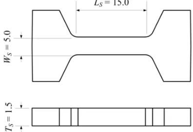
The specimen geometry used is depicted in Fig.2. With these initial geometries one can make some rough energy estimations that can be used to estimate the strain rates at which the use of the FW is effective for a particular specimen geometry and material stress-strain response. The kinetic energy that is stored in the FW is uniquely dependent on its angular velocity:
Ek =
1 2Iω
2 = 1
16mwD
2
wω2= 64πρWWDw4ω2. (1)
Figure 1. Schematic design of the flying wheel.
Figure 2. Geometry and dimensions of the specimen.
For the sake of simplicity all the elastic constants (E =210 GPa andν=0.3) as well as the mass density (ρ=7850 kg/m3) were considered to be the same for all the materials. The specimen was considered as a generic rate-independent steel with power-law hardening,
Yε¯p
=A+B ¯εnp (2)
where A=250 MPa, B=800, n=0.1 and ¯εp is the
equivalent plastic strain. Let us assume, using von Mises plasticity, that the strain energy that needs to be consumed to fully fracture the specimen is:
Es=AsLs
¯εpf
0
¯
σ(ε) d ¯εp (3)
being ¯σ the von Mises equivalent stress. Assuming an engineering failure strain of u/LS=50% an approximate
energy of 41.6 Joules is calculated to be necessary to fracture the specimen. Therefore the energy of the wheel needs to be significantly larger than that.
Given the dimensions of the wheel, for rotation frequencies of 0.1, 0.5, 1.0 and 1.5 Hz the wheel has a kinetic energy of 22.27, 556.81, 2227.27 and 5011.32 J respectively. In principle, the last three frequencies would allow the wheel to store enough energy to fracture the specimen. The first frequency however would not be enough to do it and therefore the wheel would stop rotating.
Figure 3. SDOF system representing the puller-specimen system.
3. Theoretical analysis
3.1. Problem set-up
We consider the Flying Wheel as an infinite bar with a diameter much bigger than that of the puller that travels at a velocityv and that hits the stationary puller. The flange where the impact occurs has a way smaller dimension than the rest of the components involved in the calculation so it will be neglected. The wave generated inside the puller reaches the specimen-puller interface end with velocity
v at a time LP/c and it initially is fully reflected with
a velocity twice the initial one. The time that the wave takes to do so is 2LP/c Note that c=
√
E/ρ is the elastic wave propagation velocity in the material. When the reflected wave reaches the hammer-puller contact interface the leftmost puller end detaches from the hammer as it moves with a velocity of 2v. The force applied by the specimen slows the puller down from 2v to some speed
αv until the puller is caught by the hammer again at time ti, where i is the number of contact interactions between
the hammer and the puller. It is important to note that the duration of the free-flying periods is much longer than the duration of a single wave round-trip within the puller bar. Consequently, the wave propagation within the puller will not be described and quasi-static conditions assumed instead. The set of velocity conditions of the specimen-puller interface can be written as:
u(t)=
0 0≤t<LP
c
v→2v t=LP
c
2v LP
c<t ≤3LP
c u(t) 3LP
c<t<t1 +LP
c
αv→2v−αv t=t1+LP
c 2v−αv t1+LP
c<t≤t1+3LP
c u(t) t1+3LP
c<t <t2 +LP
c. (4) Note that the same set of conditions applies again after time t2+Lp/c. In order to determine the unknown
velocity u(t) of the puller bar in the periods when it is not in contact with the hammer, a simplified single degree of freedom system representing the specimen-puller system is considered (see Fig.3). More specifically, the puller bar is considered as a lumped mass that is attached to a non-linear spring representing the specimen. The equation of motion of such system reads:
ASLS =aSlS (7)
where AS and LS are the area and gage length of the
specimen respectively, while the lower case aS and lS are
their deformed counterparts, the force in the specimen Fs
could be written as a function of the applied displacement as:
Fs{u (t)}=σ(ε) as
= A+B ln 1+u (t) Ls
n
asLs
Ls +u (t)
· (8)
The ODE was solved numerically considering the following initial conditions:
3LP
c<t <t1+LP
cu
3LP
c=2v u3LP
c=0
t1+3LP
c<t <t2+LP
c ×u
t1+3LP
c=2v−αv ut1+3LP
c=ut1+3LP
c.
(9)
3.2. Results
Equation (4) along with the non-linear boundary con-ditions (9) was solved to obtain the puller velocity history for FW rotation frequencies of 1 and 1.5 Hz. The calculations were stopped at a displacement of around 5 mm which would correspond to an engineering strain of 33%. The displacement (red) and the velocities (blue) at the specimen-puller interface obtained from solving the ODE are plotted in Fig. 4. The black curves represent the constant linear velocity of the hammer and its displacement calculated as its integral with respect time. It should be noted that such black curves would represent the puller ideal behavior as stated in the previous sub-section. In other words, it would be the behavior we sought in the design of the FW system. The solid curves correspond to the ODE solution, while the dashed curves correspond to the velocity conditions summarized Eq. (4).
The plots of Fig. 4 give a clear idea of what is happening during the specimen loading in the FW system. Regardless of the rotation frequencies, the phenomenon is basically the same. When the wave generated in the hammer-puller impact reaches the specimen-puller interface the velocity jumps from 0 to 2valmost instantly. It can also be observed that the displacement is increasing linearly with time. After that period the velocity remains constant until the reflected wave reaches the puller free end (starts the free-fly of the puller) and comes back. The displacement increases due to the velocity jump,
Figure 4. Displacement and velocity of the puller as a function
of time as a result of using the simplified model for rotational frequencies of 1.0 (a) and 1.5 Hz (b).
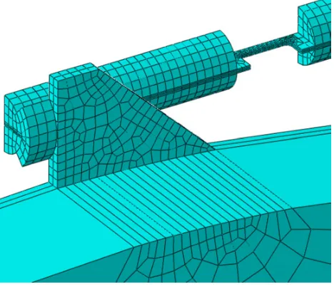
Figure 5. Finite element model of the FW system depicted in
Fig.1.
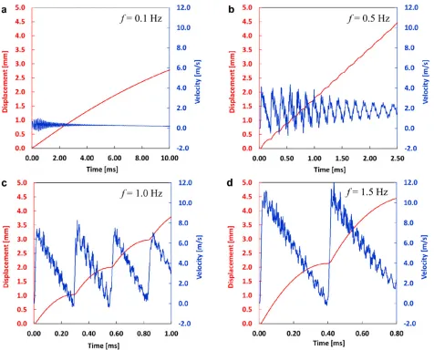
Figure 6. Velocity and displacement of the puller as a function of time obtained from the numerical simulations of the FW system of
rotation frequencies of 0.1 (a), 0.5 (b), 1.0 (c) and 1.5 Hz (d).
again and the process starts all over again. The puller free-fly period increases with increasing angular velocity as can be seen by comparing Figs. 4(a) and (b). Those longer “free-fly periods” increase the deviation of the puller displacement history from the ideal linear path, which may be seen as a loss of displacement control during the test.
4. Numerical simulations
4.1. Numerical set-up
Four numerical simulations of the FW system shown in Fig. 1 are performed. Each one of them corresponds to a specific rotational frequency: 0.1, 0.5, 1.0 and 1.5 Hz. The geometry was discretized with eight-node reduced integration elements with stiffness-based hourglass control. The specimen gage length was discretized with 0.2 mm elements, while the rest was meshed with an approximate element size of 3 mm (see Fig. 5). The specimen behavior was modelled according to what is exposed in the subsequent sub-section. The rest was considered as elastic. Due to symmetry conditions only one half of the entire system was modelled. The specimen clamping to the puller and
load cell was done sharing nodes. The displacement of the non-clamped load cell end nodes was constrained. The angular velocity was initially imposed through a coupling between the wheel and an additional rigid body that rotates at the same velocity. The rail on which the puller is mounted was simulated as a non-frictional analytical rigid surface. The contacts between surfaces were modelled employing a surface-to-surface algorithm [8]. A J2 plasticity model with associated flow rule and isotropic power-law hardening is employed to describe the specimen material.
4.2. Results
amplitude and frequency of the specimen-puller interface velocity. For very slow wheel speeds (e.g. 0.1 Hz) the displacement of the specimen-puller interface converges towards the ideal one. However, different from loading at higher speeds, a noticeable drop of the velocity is present due to the lower wheel energy. Recall that the energy of the wheel was not enough to fracture the specimen according to the energy calculation made in the previous section. Therefore, the wheel stops spinning and the displacement of the puller remains constant.
5. Conclusions
The basic working principle of the specimen loading in a tensile FW experiment has been analyzed. An analytical model is developed to predict the displacement history that is imposed onto the specimen boundaries for a FW rotating at a constant speed. Additionally, numerical simulations are performed of the same FW system for wheel rotational frequencies of 0.1, 0.5, 1.0 and 1.5 Hz to confirm the validity of the analytical model.
The analysis clearly demonstrates that the loading speed applied onto the specimen boundary by a FW system is not constant even if the wheel rotates at constant angular velocity. This is due to the necessary insertion of a short puller bar that transmits the load from the rotating wheel to the specimen boundary. For a 1.1m diameter FW system with an 80mm long puller bar and a small 15mm long steel specimen, the velocity oscillations are negligibly small in experiments with an average strain rate of 20/s. However, already at 120/s, the loading speed oscillations are very significant oscillating between 0 and 240/s at a
the French National Research Agency (Grant ANR-11-BS09-0008, LOTERIE).
References
[1] M.A. Meyers, Dynamic Behavior of Materials. (1994): John Wiley & Sons.
[2] B. Song and W. Chen, W., Split Hopkinson (Kolsky) Bar. (2011): Springer.
[3] P. Viot, F. Beani, and J.L. Lataillade, Polymeric foam behavior under dynamic compressive loading. J Mater Sci, (2005). 40(22): p. 5829–5837.
[4] R. Bouix, P. Viot, and J.-L. Lataillade, Phenomeno-logical study of a cellular material behaviour under dynamic loadings. J. Phys. IV France, (2006). 134: p. 109–116.
[5] R.R. Ambriz, C. Froustey, and G. Mesmacque, Determination of the tensile behavior at middle strain rate of AA6061-T6 aluminum alloy welds. International Journal of Impact Engineering, (2013). 60(0): p. 107–119.
[6] C. Froustey, M. Lambert, J.L. Charles, and J.L. Lataillade, Design of an Impact Loading Machine Based on a Flywheel Device: Application to the Fatigue Resistance of the High Rate Pre-straining Sensitivity of Aluminium Alloys. Exp Mech, (2007). 47(6): p. 709–721.
[7] L.W. Meyer and S. Abdel-Malek. Deformation and Ductile Fracture of a Low Alloy Steel under High Strain Rate Loading. in 2nd International Conference on High Speed Forming. (2006).