ADAPTING THE NORMALIZED CUMULATIVE
PERIODOGRAM PARAMETER-CHOICE METHOD TO THE TIKHONOV REGULARIZATION OF 2-D/TM ELECTROMAGNETIC INVERSE SCATTERING USING BORN ITERATIVE METHOD
P. Mojabi and J. LoVetri
Department of Electrical and Computer Engineering University of Manitoba
Winnipeg, MB, R3T 5V6, Canada
1. INTRODUCTION
The inverse scattering problem consists of determining the shape, location and constitutive parameters, i.e., permittivity, permeability and conductivity, of an unknown bounded object immersed in a known background medium, from the measured scattered field exterior to the object when it is irradiated by a number of known incident fields. The inverse scattering problem has been an area of interest during the last two decades due to its various applications such as medical imaging and non-destructive testing [1–7]. The research into this field has led to the development of a multiplicity of inversion algorithms; see for example [8–17]. These inversion algorithms attempt to minimize an appropriate cost-functional iteratively. Two different cost-functionals have been mostly used for formulating the inverse scattering problem [18]. The first one is the ‘conventional’ approach where the cost-functional is the discrepancy between the measured data and the predicted data augmented with an additional term to stabilize the inversion. This approach requires the solution of the forward scattering problem in each iteration. In the second approach, an error term involving the integral equation relating the fields inside the imaging domain to the constitutive parameters of the unknown object, is added to the conventional cost-functional to make a new cost-functional [9, 15]. This approach uses the Conjugate Gradient (CG) technique for minimizing the cost-functional and does not need the solution of the forward scattering problem, but the number of variables to be optimized is much larger than the conventional approach. In this paper, we use the Born Iterative Method (BIM) [11] which is based on the conventional approach to inversion. The focus of the paper is to study and suppress the inherent instability associated with the mathematical formulation of the inverse scattering problem in the framework of the BIM. The proposed algorithm is tested against the synthetic and experimental data.
ill-posed system of equations (other regularization techniques that use a penalty approach, such as the multiplicative penalty method [9, 21], are also available). The main idea behind the standard-form Tikhonov regularization is that the regularized solution, xλ, to the ill-posed
system Ax = b is taken to be the one that minimizes the functional
b−Ax22 + λ2x22, for a particular choice of the regularization parameter λ. The problem then becomes choosing an appropriate regularization parameter. Projection methods attempt to regularize by projecting the discretized problem onto a subspace having a basis that can be used to represent the solution with sufficient accuracy while maintaining stability. Some commonly used projection methods are the Truncated Singular Value Decomposition (TSVD) [22], and Krylov subspace methods [20, 23]. The hybrid methods seek to further regularize the projected problem [23, 24] because, quite often, the projection approach does not regularize the problem sufficiently.
The regularization in each of these methods usually requires the computationally expensive step of choosing the optimum regularization parameter. This is because the resulting solution can be very sensitive to the choice of the regularization parameter. In the Tikhonov method, the regularization parameter controls the weight of the penalty term, while in the projection methods, the dimension of the subspace is considered as the regularization parameter, and therefore in the hybrid methods we need two regularization parameters: one for the dimension of the subspace and the other for regularizing the projected problem. Many regularization parameter-choice methods for Tikhonov regularization have been proposed in the literature; for example, the discrepancy principle, Generalized Cross-Validation (GCV), and the
aforementioned parameter-choice methods are based on the norm of the residual vector.
For a typical inverse electromagnetic problem the norm of the noise in the measured data is not usually known and so the discrepancy principle is of little use. On the other hand, when the GCV and L -curve methods are combined with any of the Born iterative methods, they become computationally expensive because a good regularization parameter, which usually requires the Singular Value Decomposition (SVD), must be chosen at each iteration. That is, the choice of the regularization parameter for minimizingb−Ax2
2+λ2x22 whereA
is the discretization of the ill-posed operator for the problem depends onA(more specifically, it depends on the singular values ofA). In the Born iterative method, at each iteration A changes because the total field inside the imaging region is updated. Therefore at each iteration
Achanges and we should choose a new regularization parameter. It is true, that for some weakly scattering problems the change will be minor and one can keep the regularization parameter the same throughout the iterations. But in general this is not true.
In this paper, we use Tikhonov regularization in conjunction with a new parameter-choice method for solving the discretized inverse scattering problem using the BIM. This new parameter-choice method is based on the Normalized Cumulative Periodogram (NCP) of the residual vector, as opposed to just using the norm of the residual: more of the available information is used. This so-called NCP parameter-choice method was recently introduced by Hansen et al. [31] for solving discretized linear Fredholm integral equations of the first kind. The underlying idea of their method can be explained as follows: suppose that the measured data, contained in the vector b, can be modeled as the sum of an exact component ¯b, satisfying Ax¯ = ¯b where ¯x is the exact solution, and a white noise component e. Then, due to the smoothing effect of the ill-posed operator [31], the power spectrum of the exact component, i.e., ¯b, will be dominated by low frequencies whereas the power spectrum of the white noise component will have the same expected value at all frequencies. Therefore, this difference in the spectral content can be used to find a good regularization parameter for the ill-posed problem.
operating on ¯x, no longer corresponds to the exact component of the right-hand side ¯b. At any point in the iteration procedure, ¯b
may not satisfy the discrete Picard condition [32] with respect to the approximated (linearized) ill-posed operator. Thus, the NCP criteria cannot be applied to the linearized problem and it needs to be adapted for this problem. Briefly, the adaptation consists of creating a “noisy problem” by adding synthetic white noise to the right hand side of the original problem and finding the optimum regularization parameter in the noisy problem and applying it to the original problem. The linearization affects not only the NCP parameter-choice method but also both the L-curve and the GCV methods and therefore the technique described herein should be applicable to those methods.
The new procedure is applied to two different sets of problems in this paper: one based on synthetic data and the other on experimental data. For the first set, we assume that data collection is done by a set of receivers which are located on a circle around the object and that the object is illuminated by Transverse Magnetic (TM) plane-waves impinging on the object from different angles of incidence. The geometrical configuration is the same as that described in [11]. In the second set, we use measurement data collected by researchers at the Institut Fresnel for two different targets, namely FoamDielIntTM
and FoamDielExtTM [33, 35]. Here, we use single frequency data,
at 2 GHz, for reconstructing the contrast profiles of both synthetic and experimental data. We only show results for 2 GHz because the higher frequency data, provided by Institut Fresnel, is very difficult to invert using the BIM. For other inversion techniques, such as the Distorted Born Iterative Method (DBIM) [12], the NCP parameter-choice method for Tikhonov regularization which is proposed in this paper, is also applicable to the case of higher frequency and multi-frequency inversion. For the case of multi-frequency inversion the frequency hopping method can be used [34]. A review of alternative more robust inversion techniques, that have been used on the Fresnel data, such as the Multiplicative Regularized Contrast Source Inversion (MR-CSI) and the modified gradient methods, is available in [35].
2. FORMULATION OF THE LINEARIZED AND DISCRETIZED PROBLEM
The nonlinear integral equation that encapsulates the 2-D time-harmonic, scalar inverse scattering problem for transverse magnetic fields is written as
Ezs(r;k) =k02
+∞
−∞ +∞
−∞
G(r,r;k0)Ez(r;k)O(r)dxdy (1)
wherer=xax+y
ay represents the observation point in the Cartesian
coordinate system, k = kx
ax+ky
ay represents the wavevector, and
the wavenumberk0 is related to the wavevector byk0 =|k|. Ezs(r;k) is
thez-component of the scattered electric field defined as the difference between the total field and the incident field. In (1), for a non-magnetic media, O(r) = εr(r)−1 is the contrast profile, with respect to the
dielectric constant εr, that must be recovered. It will be assumed
that the scattering object is lossless for the remainder of this paper. The two-dimensional free-space Green’s function, assumingejωt
time-dependency, is given as
G(r,r;k0) =
1 4jH
(2)
0 (k0|r−r|) (2)
whereH0(2)(x) is the zeroth-order Hankel function of the second kind. Equation (1) is the basis upon which the standard domain and data equations are defined for the 2-D/TM inverse scattering problem.
For obtaining a solution for the contrast in (1), we use the BIM (described in [11]). This method proceeds by first using the Born approximation [37] to linearize the problem which is then discretized and solved for the unknown contrast using an inverse solver. The total field inside the imaging domain, corresponding to this contrast, is then computed using a moment-method forward solver based on Richmond’s method [38]. The newly updated total field, Ez(p)(r;k)
At each iteration step p, after discretizing the linearized integral equation with an approximate kernelG(r,r;k0)Ez(p)(r;k), we obtain a
discrete ill-posed system of linear equations ˜Ax=b, where ˜A∈Cm×n,
b ∈ Cm and x is to be found using an inversion technique. The matrix ˜A is a discrete representation of the linearized kernel, while
x and b are column-wise stacked representations of the 2-D discrete contrast function,O(x, y), and the measured scattered field,Ezs(x, y), respectively. Note that two errors are associated with this procedure: a linearization error as well as a discretization error. If we denote by A the discrete representation of the exact (nonlinear) kernel, i.e., the discretization of G(r,r;k0)Ez(r;k), then the difference between
A and ˜A is a representation of the linearization error. Although we don’t have access to A, obtaining a sufficiently accurate solution to the inverse problem requires that ˜A become as close as possible to A
through the BIM procedure. Thus, we expect that at later steps in the BIM procedure, the linearization error is reduced. This is essential for the inversion technique that we are applying.
3. THE GENERAL-FORM TIKHONOV REGULARIZATION INVERSE SOLVER
The pseudo-inverses of A, as well as ˜A, are unbounded due to the ill-posedness of the inverse problem. For solving the ill-posed matrix equation ˜Ax = b, we use the Tikhonov regularization method, which effectively produces a regularized pseudo-inverse operator, ˜A†λ, that is bounded, in conjunction with a parameter-choice method based on the NCP that keeps the solution as close as possible to the exact solution. The general-form Tikhonov regularization method is represented concisely as producing a solution xλ to the minimization
problem [42]
xλ = ˜A†λb = arg min x
Ax˜ −b2
2+λ
2L(x−x 0)22
= arg min
x
˜
A λL
x−
b λLx0
2
2
(3)
where λ is the regularization parameter, and L ∈ Ck×n is called the
regularization matrix which can be any matrix whose null space does not intersect with the null space ofA to ensure a unique solution [43]. The vector x0 is generally taken as a guess of the solution, and in
choose Lto be either the identity operator, or the Laplacian operator with zero boundary conditions for the unknown contrast profile. In these cases, the null space of L is trivial and does not intersect with the numerical null space of the ill-posed operator, making the solution of (3) unique. It should be mentioned that L not only controls the smoothness of the ill-posed operator but also controls the sensitivity of the solution to perturbations of both ˜A and b[44].
4. THE NCP PARAMETER-CHOICE METHOD
In this section the NCP parameter-choice method is briefly explained so that our modifications required for the method to be effective for the nonlinear inverse scattering problem can be better understood. The NCP of a vector is derived from the power spectrum of the vector as will be defined below. The main idea behind this method is to choose the largest regularization parameter λthat makes the residual vector
rλ =b−Axλ, look like white noise. We do this by starting with a large
λfor which the residual vector does not look like white noise and then reduce λ until the first instance where we have a residual vector that looks like white noise. Here “look like white noise” is defined using the Kolmogorov-Smirnov (KS) limits (to be explained below). We first express the residual vector in terms of the left singular vectors of the operatorA. Note that the SVD ofAis used only for analysis purposes and we don’t need to take the SVD of the operator in practice.
Assumed that the exact ill-posed operator,A, is known and that we can obtain its singular value decomposition A=UΣVH, where U
and V are the matrices of left and right singular vectors, ui and vi, of
the matrixA, with eachui andvicorresponding to a singular valueσi.
Here the matrix of the singular values is defined as Σ = diag{σi}. For
simplicity of the discussion, assume that L = I, the identity matrix, and x0 = 0, then the residual vector of the Tikhonov solution of
Ax=b= ¯b+ecan be written as
rλ =b−Axλ =UΛUH¯b+UΛUHe, Λ = diag
λ2 λ2+σ2
i
(4)
The vectors ¯b and e are the exact and the noise components of the right-hand side,b= ¯b+eand we are assumingeto be white noise. For the case whereL=I, in (4) the singular values will be substituted by generalized singular values of the pair (A, L) andU will be replaced by the orthonormal matrix in the decomposition ofAusing the generalized singular value decomposition of (A, L) [45].
for ill-posed problems. The regularization parameterλdetermines the “cut-off” index, kc, of this high-pass filter: the smaller the value of λ,
the larger the cut-off index. Therefore, assuming a cut-off index kc,
the first term in the residual,UΛUH¯b can be written as
n i=1 ui λ2
λ2+σ2
i
uHi ¯b
= kc i=1 ui λ2
λ2+σ2
i
uHi ¯b
+
n
i=kc+1 ui
λ2
λ2+σ2
i
uHi ¯b
≈ n
i=kc+1 ui
λ2 λ2+σ2
i
uHi ¯b
(5)
In addition, because ¯b satisfies the discrete Picard condition [32], i.e.,
|uHi ¯b| for anything but the first few indices will decay to zero faster than the singular values σi (or the generalized singular values when
L = I), Equation (5) is almost zero for an appropriate choice of the parameterkc, which itself depends on the regularization parameterλ.
That is, considering the high-pass filter characteristic of Λ and the discrete Picard condition, it can be concluded that as we decrease λ, we will reach a cut-off index for the filter which suppresses all the significant components of ¯b in the SVD basis. Using a cut-off index that suppresses all of the significant components of ¯b in the residual means that we’ve used as much information as possible in the solution, and choosing the smallest such index, i.e., largest λ, ensures a stable solution (giving an acceptable trade-off between the regularization and perturbation errors). The regularization parameter corresponding to this cut-off index can be considered as the optimum regularization parameter, λopt, because it singles out the most stable solution whose
residual does not have any dominant component of ¯b. The residual vector for this optimum regularization parameter will be
rλopt =UΛoptU
H¯b+UΛ
optUHe≈UΛoptUHe, Λopt = Λ|λ=λopt (6) Thus, forλ=λopt, the residual vector will be dominated byUΛoptUHe.
Considering the fact that the noise on the right-hand side, e, is white noise with a standard deviation of, say, η, its covariance matrix will be cov{e}=η2I. The covariance matrix of the vector UΛUHe can be calculated as
cov{UΛUHe}=UΛUHcov{e}UΛUH =η2UΛ2UH ≈η2Ikc (7)
where Ikc is the identity matrix with the first kc diagonal elements
behaves statistically like white noise for ill-posed problems. Therefore, considering this fact as well as the fact that the dominant values of
|uHi ¯b| correspond only to the first few indices, one can conclude that the optimum regularization parameter can be considered as the largest
λ, i.e., the smallest cut-off index, which makes the residual vector,rλ,
behaves like white noise.
The metric that is used to see if the residual “looks” like white noise is the NCP of the residual. So the standard NCP parameter-choice method starts with a large λ— in which case the NCP of the residual vector will look like that of the data — and therefore we have most of the data information left in the residual. We then decrease
λuntil the NCP of the residual first becomes like that of white noise (i.e., a curve between the KS limits for white noise [46], which are bounds around a straight line). Once this happens, we can be sure that all the important information available in ¯b has been used in calculating xλ, even though we don’t have access to ¯b. Notice that if
we decreaseλfurther, the residual is still white noise (or slightly high-pass filtered white noise) but the solution is more likely to be unstable due to perturbation errors.
One note regarding this use of the NCP parameter-choice method is that NCP is usually defined for real vectors — because it is generally used as a statistical time-series analysis tool [46] — but here we use the same definition for the NCP of a complex vector. Denoting the power spectrum of the residual as P ∈ Rn, the components of the NCP vector,C ∈Rn−1, are calculated as
Ci= [P1−P1]−1
i+1
j=2
Pi, i= 1,2, . . . , n−1 (8)
whereP1 is the first (or DC) component of the vector P. In our case,
the KS-limit lines, as a function of index i, are given as i/n−1±δ
5. USING THE NCP PARAMETER-CHOICE METHOD IN THE BORN ITERATIVE METHOD
In each iteration of the Born iterative method a discrete ill-posed system of equations, ˜Ax = b is constructed where ˜A is a linearized approximation to the exact ill-posed operator. We can express ˜A =
A+E whereE is an error matrix due to the use of the approximated total electric field, instead of the unknown exact field inside the imaging domain. This error could be quite considerable in the first iteration and gradually decreases in subsequent iterations, but the right-hand side (i.e., the measured data) stays the same for all iterations. The effect of this linearization error can be evaluated as follows.
We first note that, using (4) in summation form with ˜U instead of
U, the residual vector at each iteration of the BIM can be written as
rλ= n i=1 ˜ ui λ2 λ2+ ˜σ2
i
˜
uHi ¯b+
n i=1 ˜ ui λ2 λ2+ ˜σ2
i
˜
uHi e (9)
where ˜ui is a left singular vector of the linearized discrete operator ˜A.
For a sufficiently large value of λ, the second term on the right-hand side of (9) behaves statistically like white noise because it satisfies (7) with a small kc. On the other hand, although ¯b is such as to satisfy
the discrete Picard condition with respect toA, but it does not satisfy the discrete Picard condition with respect to the linearized operator,
˜
A. Therefore, ˜uH
i ¯bcannot be filtered out with any choice ofλ. So it is
not possible to apply the NCP criterion as the NCP of the residual can never be made to look like that of white noise. This can be explained as follows. Assume that at the pth iteration of the BIM, we have ˜Ax = b = ¯b+e. The exact data ¯b can be decomposed into two different terms: ¯b= ˜b+esuch that ˜bis the right-hand side of the equation ˜Ax= ˜b. Unfortunately, we do not have access to ˜b, onlyb. So we end up solving ˜Ax=b= ˜b+δ+evia regularization, which means that we minimize (3) with the corresponding residual expressed as
rλ = n i=1 ˜ ui λ2 λ2+ ˜σ2
i
˜
uHi ˜b+
n i=1 ˜ ui λ2 λ2+ ˜σ2
i
˜
uHi δ+
n i=1 ˜ ui λ2 λ2+ ˜σ2
i
˜
uHi e (10)
should be noted that the presence ofδ is an essential part of the BIM process for converging to the solution but it makes the finding of the regularization parameter using any of the standard parameter-choice methods, namely GCV and the L-curve methods, as well as the NCP parameter-choice method, difficult.
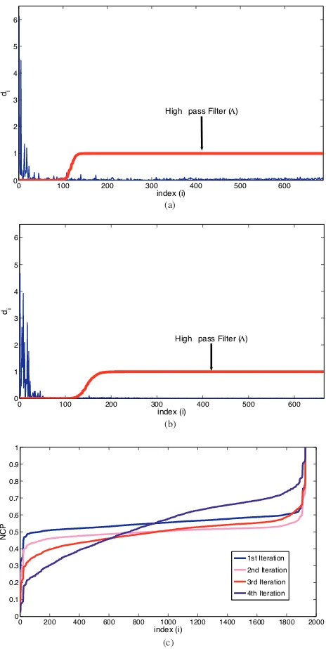
In Figure 1(a),di =|u˜Hi b|for 1≤i≤665are plotted for the first
iteration of the BIM for the FoamDielIntTM profile (to be described later) where n = 1849. Also, the high-pass filter Λ corresponding to
λ = 10−4 is shown. It can be seen from Figure 1(c) that even for such a very small λ, it is not possible to fit the NCP of the residual into the Kolmogorov-Smirnov limits because of the small peaks in the pass-band of the filter which are due to |u˜H
i δ|. Figure 1(b) shows
the same plot corresponding to the fourth iteration of the BIM. As expected, ˜A is now closer to A compared to the first iteration and therefore, δ is smaller. So, the NCP of the residual for this iteration corresponding to the same λ is closer to the NCP of white noise. In Figure 1(c), the NCP of the residual for all four iterations of the BIM for the sameλ, i.e.,λ= 1e−4, are shown. It should be noted that the optimum regularization parameters for these four different iterations have been found using the adapted NCP method (to be explained in Sec. 5.1) andλ= 1e−4 has been chosen just for the comparison. With each iteration, the exact ill-posed operator is better approximated and therefore the NCP of the residual will tend to be closer to the NCP of white noise but can never be made to fit into the Kolmogorov-Smirnov limits when the approximated kernel is not close enough to the exact kernel.
5.1. Adapting the NCP Method for Use with the BIM
The underlying assumption for using standard parameter-choice methods, like the NCP method, in conjunction with Tikhonov regularization is that the right-hand side should consist of two parts: the first part must satisfy the discrete Picard condition and the second part must be white noise (or if the noise is non-white, an estimation to its covariance matrix must be known). In different iterations of the BIM, the right-hand side consists of three parts: ˜bwhich satisfies the discrete Picard condition,ewhich is white noise andδ which does not satisfy the discrete Picard condition and also it is not white noise. Therefore, standard parameter-choice methods are not applicable to this problem because of the presence ofδ.
0 100 200 300 400 500 600 0
1 2 3 4 5 6
di
index (i)
High pass Filter (Λ)
0 100 200 300 400 500 600
0 1 2 3 4 5 6
index (i) di
High pass Filter (Λ) (a)
(b)
0 200 400 600 800 1000 1200 1400 1600 1800 2000
0 0.1 0.2 0.3 0.4 0.5 0.6 0.7 0.8 0.9 1
index (i)
NCP
1st Iteration
2nd Iteration 3rd Iteration
4th Iteration
(c)
Figure 1. (a) di = |u˜Hi b| vs. 1 ≤ i ≤ 665where n = 1849 for the
first iteration of the BIM for FoamDielInt and the high-pass filter, Λ, corresponding toλ= 10−4, (b) the same plot corresponding to the
not restricted to only the first few left singular vectors and cannot be suppressed by Λ. The components of δ corresponding to first few left singular vectors should not be in the residual as they are necessary for converging to the true profile. However, the remaining components of δ should remain in the residual vector because otherwise they will produce an unstable solution. For adapting the NCP method for the BIM, we try to modify the right-hand side in such a way to satisfy the underlying assumption of the standard parameter-choice methods.
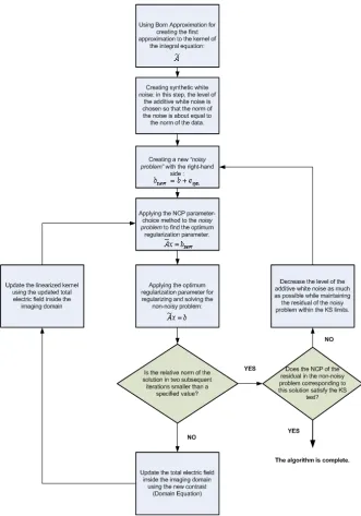
To solve this problem, we create a new“noisy problem” by adding synthetic white noise, esyn, to the right hand side of the equation
˜
Ax=b in the first step of the BIM, that is, the Born approximation. This creates a new equation for the noisy problem, ˜Ax = bnew =
˜b+δ+e+esyn, which is such that those components of ˜uH
i δ, that are not
among the first few left singular vectors, are insignificant compared to ˜
uH
i (e+esyn) which does have an NCP that looks like white noise. (The
initial amount of noise that is added is chosen so that the norm of the additive noise, esyn2, is about equal to the norm of the data, b2,
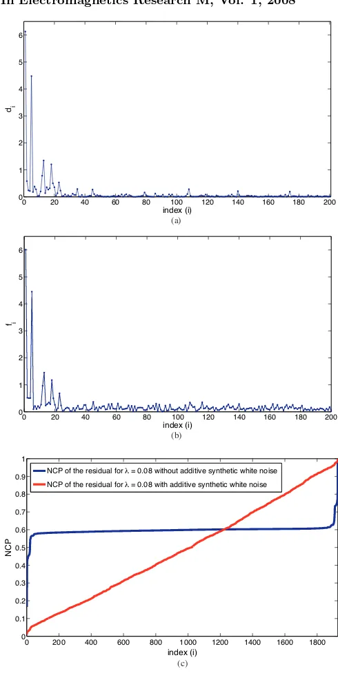
guaranteeing that the components of ˜uHi δ are insignificant compared to ˜uHi (e+esyn) except for first few components of ˜uHi δ). For example,
the |u˜Hi b| terms for the first iteration of the FoamDielIntTM where 1 ≤ i ≤ 200 and n = 1849 are shown in Figure 2(a). These can be compared with thefi =|u˜Hi bnew|shown in Figure 2(b) where the norm
of the additive white noise has been set about equal to the norm of the data. As can be seen from the figure, the significant components of |u˜H
i b| are not significantly affected with the addition of noise, but
looking at Figure 2(c), where the NCP of the residual corresponding to
λ= 0.08 is shown for these two cases, the noisy residual can be made to look like white noise.
This allows us to apply the NCP parameter-choice method to the noisy problem ˜Ax =b+esyn at any iteration of the BIM to find the
0 20 40 60 80 100 120 140 160 180 200 0
1 2 3 4 5 6
index (i) di
0 20 40 60 80 100 120 140 160 180 200 0
1 2 3 4 5 6
index (i) fi
(a)
(b)
0 200 400 600 800 1000 1200 1400 1600 1800 0
0.1 0.2 0.3 0.4 0.5 0.6 0.7 0.8 0.9 1
index (i)
NCP
NCP of the residual for λ = 0.08 without additive synthetic white noise
NCP of the residual for λ = 0.08 with additive synthetic white noise
(c)
Figure 2. (a) di = |u˜iHb| vs. 1 ≤ i ≤ 200 for the first iteration of
the BIM for FoamDielInt, (b) fi = |u˜iHbnew| vs. 1 ≤ i ≤ 200 for the
termination condition). But if the NCP of the residual for the non-noisy problem does not satisfy the KS test (meaning that the solution is over-smooth), the level of the additive noise is decreased as much as possible while maintaining the NCP of the residual for the noisy problem within the KS limits and the same algorithm is applied until these two different termination conditions are satisfied. The flowchart of this algorithm is shown in Figure 3.
We have found that in running this algorithm it is sufficient to use a significance level of 5% for the KS limits when using the noisy problem to find the optimum regularization parameter and then to increase the significance level (say, to 10%) for the second termination condition. Slightly varying the significance level of the KS limits seems to affect the rate of convergence but the final solution generally remains the same.
6. NUMERICAL RESULTS
6.1. Imaging Results Based on Synthetic Data
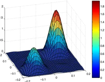
In this section we present the results for two cases where the scattering data is obtained synthetically from a numerical solver. The synthetic data was produced by a method of moments (MoM) solver with triangular meshes (3448 triangular meshes over the imaging domain) and white noise was added such that the signal to noise ratio is SNR = b¯2/e2 = 10. The two scattering cases consist of (i)
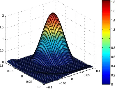
a sinusoidal contrast with amplitude of 2.0, shown in Figure 4(a) and (ii) two spatially separated sinusoidal contrasts of amplitudes 2.0 and 1.0, shown in Figure 5(a). Figures 4(b), 4(c), 5(b) and 5(c) show the resulting reconstruction using both the identity and the Laplacian operators as the regularization matrices for these two synthetic cases. In the BIM, the forward solution was obtained by Richmond’s method [38] using a pulse basis on a square mesh covering the imaging domain (The number of pulses over the imaging domains is 40×40).
-0.1 -0.05 0 0.05 0.1 -0.1 -0.05 0 0.05 0.1 0 0.5 1 1.5 2 0 0.2 0.4 0.6 0.8 1 1.2 1.4 1.6 1.8 2 -0.1 -0.05 0 0.05 0.1 -0.1 -0.05 0 0.05 0.1 0 0.5 1 1.5 2 0.2 0.4 0.6 0.8 1 1.2 1.4 1.6 1.8 (a) (b) -0.1 -0.05 0 0.05 0.1 -0.1 -0.05 0 0.05 0.1 0 0.5 1 1.5 2 0 0.2 0.4 0.6 0.8 1 1.2 1.4 1.6 1.8 (c)
Figure 4. First synthetic test case (a) true profile, sinusoidal profile with peak-permittivity is 3.0 (contrast is 2.0), (b) reconstruction with
L=I, (c) reconstruction withL the Laplacian.
10 (see Figure 5b). In Figure 7, the NCP of bnew as well as the
NCP of a few residual vectors corresponding to different regularization parameters are shown for the first test case. As can be seen in Figure 7, for large values of λ the NCP of the residual looks like the NCP of
bnew, showing that we have not used all of the available information
in reconstructing the profile. As λ is decreased, less information is included in the residual and more information goes into the solution. The first NCP which fits the Kolmogorov-Smirnoff limits is the NCP corresponding toλ= 0.02.
-0.2 -0.1 0 0.1 0.2 -0.2 0 0.2 0 0.5 1 1.5 2 0 0.2 0.4 0.6 0.8 1 1.2 1.4 1.6 1.8 2
-0.2 -0.1 0
0.1 0.2 -0.2 0 0.2 0 0.5 1 1.5 2 0 0.2 0.4 0.6 0.8 1 1.2 1.4
-0.2 -0.1 0
0.1 0.2 -0.2 0 0.2 0 0.5 1 1.5 2 0 0.2 0.4 0.6 0.8 1 1.2 1.4 1.6 1.8 (a) (b) (c)
Figure 5. Second synthetic test case (a) true profile, two sinusoidal profiles with peak-contrast equal 2.0 and 1.0, (b) reconstruction with
L=I, (c) reconstruction withL the Laplacian.
2 1 0 0.1 0.2 2 1 0 0.1 0.2 0 0.5 1 1.5 2 0 0.2 0.4 0.6 0.8 1 1.2 1.4 1.6 1.8
Figure 6. Reconstruction of the second synthetic test case usingL=I
0 200 400 600 800 1000 1200 1400 1600 0.1
0.2 0.3 0.4 0.5 0.6 0.7 0.8 0.9 1
index (i)
NCP of b
new
0 200 400 600 800 1000 1200 1400 1600
0 0.1 0.2 0.3 0.4 0.5 0.6 0.7 0.8 0.9 1
index (i)
NCP of the residual vector (r
λ
)
KS limit
KS limit λ = 3.0 λ = 0.2 λ = 0.1 λ = 0.08 λ = 0.05 λ = 0.02 λ = 1e&5 (a)
(b)
Figure 7. (a) The NCP of bnew, (b) The NCP of the residual vector
corresponding to seven different regularization parameters.
parameter as compared to the NCP method. For example, in the Born approximation of the first test case, the modifiedL-curve method chooses λ = 0.013 as the optimum regularization parameter whereas the NCP method chooses λ = 0.020. In Figure 8, we’ve plotted the
L-curve for the Born approximation of the first test case using 100 differentλ’s (λNCPis the regularization parameter chosen by the NCP
method). The fact that two different parameter-choice methods choose two different regularization parameters simply reflects the fact that there is no unique solution to the inverse problem. The reconstruction of the first synthetic data usingL-curve has been shown in Figure 9 for the case L=I. For our implementation of the BIM, the result using
100.25 100.23 100.21 100.19 100.17 102
residual norm
solution norm
Regularization parameter
chosen by the L-curve method: λc
Regularization parameter
chosen by the NCP method: λNCP
λ1 λ100
-- - -
-Figure 8. Comparison between the regularization parameters chosen by the L-curve and the NCP methods corresponding to the first iteration of the BIM for the first synthetic test case.
1
0 0.05
0.1
1 0 0.05 0.1
0 0.5 1 1.5 2
0 0.2 0.4 0.6 0.8 1 1.2 1.4 1.6 1.8
Figure 9. Reconstruction of the first synthetic case withL=I using
L-curve method.
6.2. Imaging Results Based on the Experimental Fresnel Data
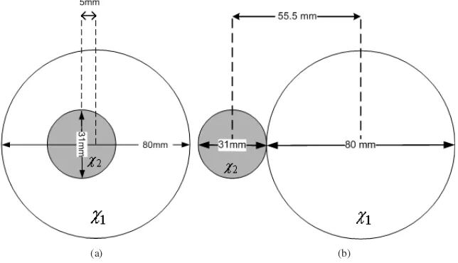
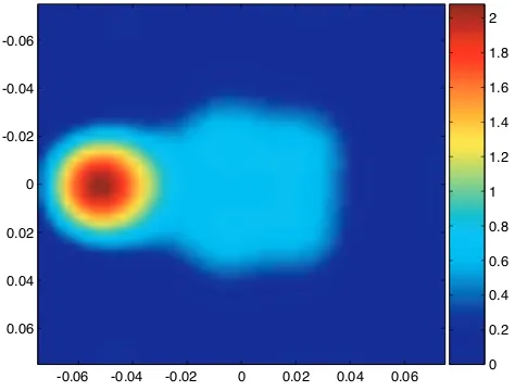
geometries are available, but here we show the reconstructions for two geometries which contain only lossless dielectrics: (i)FoamDielIntTM: a cylinder of diameterda= 31 mm with contrastχ2 = 2.0±0.30, inside
a cylinder of diameter db = 80 mm with contrast χ1 = 0.45±0.15,
with the inner cylinder off-set by 5mm; and (ii) FoamDielExtTM: the same as (i) but with the smaller cylinder located external to the larger cylinder and butted against it. These geometries are shown in Figure 10.
(a) (b)
Figure 10. True profiles for the two Fresnel cases considered: (a)
FoamDielInt, (b)FoamDielExt.
The inversion of both cases, using the NCP method, was performed using single-frequency 2 GHz TM scattering data which was calibrated for an equivalent plane-wave incident field. The bistatic scattering data was taken for 8 transmitter positions equally spaced every 45◦ around the scatterer, and 241 receiver locations, for each transmitter, equally spaced every 1◦ around the scatterer with no receiver closer than 60◦ from the transmitter. The receivers and transmitters were placed on a circle having a radius of 1.67 m, all in the same horizontal plane. The imaging domain is a 0.15×0.15m2 square centered at the center of the receiver circle. Details of the measurement and calibration procedure can be found in [33]. The forward solution of the BIM was obtained by Richmond’s method [38] using a pulse basis on a square mesh covering the imaging domain (The number of pulses over the imaging domains is 43×43.)
-0.06 -0.04 -0.02 0 0.02 0.04 0.06 -0.06
-0.04
-0.02
0
0.02
0.04
0.06
0 0.25 0.5 0.75 1 1.25 1.5 1.75 2 2.25 2.5
Figure 11. Reconstruction ofFoamDielInt.
-0.06 -0.04 -0.02 0 0.02 0.04 0.06
-0.06
-0.04
-0.02
0
0.02
0.04
0.06
0 0.2 0.4 0.6 0.8 1 1.2 1.4 1.6 1.8 2
Figure 12. Reconstruction ofFoamDielExt.
the focus of this paper is the effectiveness of the NCP method as a parameter-choice method and inversion results using single frequency inversions are adequate for this purpose. The use of our NCP method as well as other parameter choice methods in conjunction with more robust inversion methods such as DBIM and Newton-based optimization methods is a subject for a future paper.
7. CONCLUSIONS
The NCP parameter-choice method presented by Hansen et al. [31] has been adapted for solving the nonlinear 2-D/TM electromagnetic inverse scattering problem using the BIM. As for the original NCP parameter-choice method, because it is based on the FFT, and the SVD of the matrix does not need to be computed, the method is computationally efficient. As was pointed out by Hansen, the NCP method works for discretized linear Fredholm integral equations of the first kind because of the fact that the data vector for such problems will be dominated by low-frequency components in the discrete Fourier basis and the NCP of the residual above that low-frequency cut-off (determined by the regularization parameter) will look like that of white noise. For the nonlinear scattering problems considered here, the method must be adapted because the linearization of the kernel in the BIM introduces an error in the discretized operator that contributes energy to the residual across the whole frequency band and above the low-frequency cut-off the residual no longer has a NCP that looks like that of white noise. The adapted NCP method introduces additive white noise so that this error energy above the cut-off is dominated by the additive noise and therefore it can still be used as a parameter choice method. A procedure for reducing the additive white noise within the BIM has been given so that over-smoothing is avoided.
ACKNOWLEDGMENT
The authors would like to acknowledge the financial support of the Natural Sciences and Engineering Research Council of Canada and we would also like to thank Prof. P. C. Hansen for making us aware of his work on the NCP method. We also acknowledge the help of Mr. C. Gilmore for his assistance in providing the synthetic data and calibrating the Fresnel data.
REFERENCES
1. Semenov, S. Y., V. G. Posukh, A. E. Bulyshev, and T. C. Williams, “Microwave tomographic imaging of the heart in intact swine,” Journal of Electromagnetic Waves and
Applications, Vol. 20, 873–890, 2006.
2. Guo, B., Y. Wang, and J. Li, “Microwave imaging via adaptive beamforming methods for breast cancer detection,” Journal of
Electromagnetic Waves and Applications, Vol. 20, No. 1, 53–63,
2006.
3. Yan, L. P., K. M. Huang, and Liu C. J., “A noninvasive method for determining dielectric properties of layered tissues on human back,” Journal of Electromagnetic Waves and Applications, Vol. 21, 1829–1843, 2007.
4. Huang, K., X. B. Xu, and L. P. Yan, “A new noninvasive method for determining the conductivity of tissue embedded in multilayer biological structure,” Journal of Electromagnetic
Waves and Applications, Vol. 16, 851–860, 2002.
5. Davis, S. K., E. J. Bond, X. Li, S. C. Hagness, and B. D. van Veen, “Microwave imaging via space-time beamforming for early detection of breast cancer: Beamformer design in the frequency domain,” Journal of Electromagnetic Waves and Applications, Vol. 17, No. 2, 357–381, 2003.
6. Bindu, G., A. Lonappan, V. Thomas, C. K. Aanandan, K. T. Mathew, and S. J. Abraham, “Active microwave imaging for breast cancer detection,”Progress In Electromagnetics Research, PIER 58, 149–169, 2006.
7. Weedon, W. H., W. C. Chew, and P. E. Mayes, “A step-frequency radar imaging system for microwave nondestructive evaluation,”
Progress In Electromagnetics Research, PIER 28, 121–146, 2000.
9. Van den Berg, P. M. and A. Abubakar, “Contrast source inversion: State of art,” Progress in Electromagnetics Research, PIER 34, 189–218, 2001.
10. Habashy, T. M. and A. Abubakar, “A general framework for constraint minimization for the inversion of electromagnetic measurements,”Progress in Electromagnetics Research, PIER 46, 265–312, 2004.
11. Wang, Y. M. and W. C. Chew, “An iterative solution of two-dimensional electromagnetic inverse scattering problem,” Int. J.
Imaging Syst. Technol., Vol. 1, 100–108, 1989.
12. Chew, W. C. and Y. M. Wang, “Reconstruction of two-dimensional permittivity distribution using the distorted Born iterative method,”IEEE Transactions on Medical Imaging, Vol. 9, 218–225, 1990.
13. Habashy, T. M. and R. J. Mitra, “On some inverse methods in electromagnetics,” Journal of Electromagnetic Waves and
Applications, Vol. 1, 25–58, 1987.
14. Rekanos, I. T., “Time-domain inverse scattering using Lagrange multipliers: An iterative FDTD-based optimization technique,”
Journal of Electromagnetic Waves and Applications, Vol. 17,
No. 2, 271–289, 2003.
15. Kleinman, R. E. and P. M. van den Berg, “A modified gradient method for two-dimensional problems in tomography,”Journal of
Computational and Applied Mathematics, Vol. 42, 17–35, 1992.
16. Takenaka, T., H. Jia, and T. Tanaka, “Microwave imaging of electrical property distributions by a forward-backward time-stepping method,” Journal of Electromagnetic Waves and
Applications, Vol. 14, No. 12, 1609–1626, 2000.
17. Belkebir, K., S. Bonnard, F. Pezin, P. Sabouroux, and M. Saillard, “Validation of 2D inverse scattering algorithms from multi-frequency experimental data,”Journal of Electromagnetic Waves
and Applications, Vol. 14, No. 12, 1637–1667, 2000.
18. Zaeytijd, J. D., A. Franchois, C. Eyraud, and J. M. Geffrin, “Full-wave three-dimensional micro“Full-wave imaging with a regularized Gauss-Newton method — Theory and experiment,” IEEE
Transactions on Antennas and Propagation, Vol. 55, No. 11, 2007.
19. Tikhonov, A. N. and V. Y. Arsenin,Solution of Ill-posed Problems, John Wiley & Sons, New York, 1977.
20. Hansen, P. C., Rank-deficient and Discrete Ill-posed Problems, SIAM, Philadelphia, 1998.
H. Braunisch, “A multiplicative regularization approach for deblurring problems,” IEEE Transactions on Image Processing, Vol. 13, No. 11, 1524–1532, 2004.
22. Hansen, P. C., “Truncated singular value decomposition solutions to discrete ill-posed problems with ill-determined numerical rank,”
SIAM J. Sci. Stat. Comput., Vol. 11, 503–518, 1990.
23. Kilmer, M. E. and D. P. O’Leary, “Choosing regularization parameters in iterative methods for ill-posed problems,” SIAM
J. Matrix. Anal. Appl., Vol. 22, 1204–1221, 2001.
24. O’Leary, D. P. and J. A. Simmons, “A bidiagonalization-regularization procedure for large scale discretization of ill-posed problems,” SIAM J. Sci. Statist. Comput., Vol. 2, 474–489, 1981. 25. Morozov, V. A.,Methods for Solving Incorrectly Posed Problems,
Springer-Verlag, New York, 1984.
26. Hansen, P. C., “Analysis of discrete ill-posed problems by means of the L-curve,” SIAM Review, Vol. 34, 561–580, 1992.
27. Hansen, P. C. and D. P. O’leary, “The use of the L-curve in the regularization of discrete ill-posed problems,” SIAM J. Sci.
Comp., Vol. 14, 1487–1503, 1993.
28. Golub, G., M. Heath, and G. Wahba, “Generalized cross-validation as a method for choosing a good ridge parameter,”
Technometrics, Vol. 21, 215–223, 1979.
29. Iwama, N., M. Yamaguchi, K. Hattori, and M. Hayakawa, “GCV-aided linear reconstruction of the wave distribution function for the ground-based direction finding of magnetospheric VLF/ELF waves,” Journal of Electromagnetic Waves and Applications, Vol. 9, No. 5–6, 757–782, 1995.
30. Belge, M., M. E. Kilmer, and E. L. Miller, “Efficient determination of multiple regularization parameters in a generalized L-curve framework,”Inverse Problems, Vol. 18, 1161–1183, 2002.
31. Hansen, P. C., M. E. Kilmer, and R. H. Kjeldsen, “Exploiting residual information in the parameter choice for discrete ill-posed problems,” BIT Numerical Mathematics, Vol. 46, 41–59, 2006. 32. Hansen, P. C., “The discrete picard condition for discrete ill-posed
problems,” BIT, Vol. 30, 658–672, 1990.
33. Geffrin, J. M., P. Sabouroux, and C. Eyraud, “Free space experimental scattering database continuation: Experimental set-up and measurement precision,”Inverse Problems, Vol. 21, S117– S130, 2005.
Microwave and Guided Wave Letters, Vol. 5, No. 12, 1995. 35. Guest Editors’ Introduction, “Testing inversion algorithms against
experimental data: Inhomogeneous targets,” Inverse Problems, S1–S3, 2005.
36. Zha, H. and P. C. Hansen, “Regularization and the general Guass-Markov linear model,”Math. Comp., Vol. 55, 613–624, 1990. 37. Born, M. and E. Wolf,Principles of Optics, Cambridge University
Press, Cambridge, 1999.
38. Richmond, J. H., “Scattering by a dielectric cylinder of arbitrary cross section shape,” IEEE Trans. Antennas. Propag., Vol. 13, 334–341, 1965.
39. Volakis, J. L. and K. Barkeshli, “Applications of the conjugate gradient FFT method to radiation and scattering,” Progress In
Electromagnetics Research, PIER 05, 159–239, 1991.
40. Tran, T. V. and A. McCowen, “A unified family of FFT-based methods for dielectric scattering problems,” Journal of
Electromagnetics Waves and Applications, Vol. 7, No. 5, 739–763,
1993.
41. Peng, Z. Q. and A. G. Tijhuis, “Transient scattering by a lossy dielectric cylinder: Marching-on-in-frequency approach,”Journal
of Electromagnetics Waves and Applications, Vol. 8, No. 8, 973–
972, 1994.
42. Hansen, P. C., “Numerical tools for analysis and solution of fredholm integral equation of the first kind,” Inverse Problems, Vol. 8, 849–872, 1992.
43. Engl, H. W., M. Hanke, and A. Neubauer, Regularization of
Inverse Problems, Kluwer Academic Publishers, Dordrecht, 2000.
44. Hansen, P. C., “Perturbation bounds for discrete Tikhonov regularization,”Inverse Problems, Vol. 5, L41–L44, 1989.
45. Hansen, P. C., “Regularization, GSVD and truncated GSVD,”
BIT, Vol. 29, 491–594, 1989.