Electrical Capacitance Volume Tomography: A Comparison between
12- and 24-Channels Sensor Systems
Aining Wang1, Qussai M. Marashdeh2, Fernando L. Teixeira3, *, and Liang-Shih Fan1
Abstract—Spatial resolution represents a key performance aspect in electrical capacitance volume tomography (ECVT) systems. Factors affecting the resolution include the “soft-field” nature of ECVT, the number of capacitance channels used, the ill-conditioned nature of the imaging reconstruction problem, and the signal-to-noise ratio of the measurement apparatus. In this study, the effect of choosing different numbers of capacitance plates on the performance of ECVT is investigated experimentally. Specifically, two ECVT sensors with 12 and 24 capacitance channels but covering equal volumes of a cylinder are used to examine the resulting impact on the image resolution.
1. INTRODUCTION
Electrical capacitance tomography (ECT) sensors have been widely used in industrial process monitoring and multiphase flow applications including chemical processes, for example [1–4]. More recently, direct three-dimensional (3D) imaging systems based upon volumetric capacitance sensor measurements have been developed, constituting what has become known as Electrical Capacitance Volume Tomography (ECVT) [5–8]. Capacitance plates employed in ECVT yield inherent 3D sensitivity matrix maps whereby volumetric images can be reconstructed. A key feature of ECVT resides in its capability of reconstructing volume imagesdirectly, that is, without the need for any spatial averaging or interpolation of two-dimensional (2D) images (“slices”). This is especially important because capacitance sensors are typically made of elongated plates to ensure stable signal measurements from minimum single-to-noise (SNR) requirements, and 2D tomograms slices obtained from such traditional ECT sensors represent only an average result along the full axial length of the plates. Consequently, any resulting 3D interpolations taken from a collection of such 2D tomograms are expected to provide a poor representation of flow features in the axial direction.
Research on improving the imaging resolution in ECT and ECVT has focused primarily on image reconstruction algorithms and techniques [9–12]. Considerable less attention has been given to increasing the number of independent measurement channels (i.e., by considering different capacitance plate shapes, arrangements, and number). The trade-off between number of channels and the system acquisition complexity was briefly discussed [13]. The effect of number of electrodes on ECT image quality was evaluated in [14]. In particular, the authors have concluded that increasing the number of capacitance plates beyond the (conventionally used) number of 12 in ECT does little to improve quality of reconstructed image. Here, we show that these conclusions do not translate to ECVT. As shown below, the impact of further increasing the number of channels on the ECVT imaging resolution is considerably more pronounced in the volumetric case because more freedom is available on the design and spatial arrangement of the capacitance plates along its two-dimensional domain boundary.
Received 14 January 2015, Accepted 10 February 2015, Scheduled 19 February 2015
* Corresponding author: Fernando Lisboa Teixeira ([email protected]).
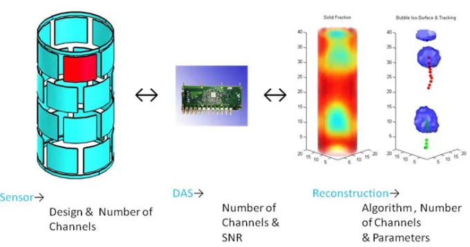
Figure 1. Schematics of an ECVT system, illustrating the three basic components that impact image resolution. The total number of channels plays a primary role in all three components.
2. ECVT SYSTEM COMPONENTS AND RESOLUTION
ECT and ECVT systems in general are studied by breaking down the system into its three basic components: (1) sensors, (2) data acquisition hardware, and (3) image reconstruction algorithms. In capacitance tomography, most of the efforts to enhance image resolution have been by far focused on the third component above. This strategy is providing ever diminishing returns as the quality of reconstructed images using different state-of-the-art reconstruction algorithms are in closer order. Since all three basic components above work in tandem to produce a given resolution, it is clear that further improvements in image quality should be sought using a more integrated approach. In Figure 1, a typical ECVT system is illustrated along with the key ingredients impacting each component and the final image resolution. From an inverse problem prospective, an increase in the number of “independent measurements” is the key for increasing the final image resolution. ECVT sensor hardware design can play a major role in determining the degree of ill-conditioning of the associated sensitivity matrix, with more “independent” measurements leading to a better conditioning of the imaging problem. The most direct route to achieve this is to increase the number of capacitance plates. However, this necessitates (1) a corresponding increase in the number of capacitance channels in the data acquisition chain and (2) a smaller area for each capacitance plate. Both these facts cause SNR degradation. Because of this, it is assumed that an increase in number of channels beyond a certain number does not have a significant impact on image quality. Historically, this limit has been assumed to be about 12 sensors and has arisen from the very limited flexibility provided by 2D ECT sensor systems in both designing and arranging the plates along the azimuth angle. In this work, we show that this low limit does not apply to ECVT due to the enhanced flexibility for the deployment of the capacitor plates around the imaging domain, and that there is a substantial gain in resolution by going from a system with 12 channels (plates) to a system with 24 channels even as the imaging domain volume remains the same.
3. ECVT SENSORS
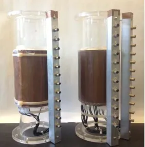
Figure 2. Two ECVT sensors of 12 and 24 plates covering the same imaging volume.
(a) (b)
Figure 3. (a) 12-channels ECVT sensor design. (b) 24-channels ECVT sensor design.
Each plate here is of 41 mm height and 50.8 mm in width, conforming to the cylindrical shape of the column. Each plate is surrounded from all sides with a rectangular strip of ground trace with 4 mm width. The distance between the ground trace and the edges of the plate is also 4 mm from all sides. The plates were fixed on the outside wall of the column, which is of 6.35 mm in thickness. The column wall dielectric constant was around 2. For proper comparison, both ECVT systems are designed to image the same volume and an identical reconstruction algorithm [15] is employed in both cases.
In both sensors, the plates are shifted halfway with respect to the plate width from one plane to another, in a staggered arrangement as seen in Figure 3. While each plate of the 24-channels system is half the size of those in the 12-channels system, the 24-channels system plates are only 30% shorter in length and 28% shorter in width. This distinction is important as it implies that shrinkage in plate area does not correspond linearly to degradation in SNR in the 3D case. To better illustrate this point, one can consider two plates in the first and third layers of the 12-channels sensors and the 24-channels sensor that are aligned vertically. For both sensors, the portions of the plates that are closer to each other have a greater effect on the capacitance measurements. Moreover, reducing thelength of a sensor plate would bring plates from different layers closer to each other. Thus, the reduction in the area of the 3D sensor plates resulting from an increase in the number of channels is partially compensated by the fact that such area reduction can be mostly associated to those regions of the plates that have comparatively less effect on the measured capacitance signals.
(a) Electrodes 1 and 3 in 12-channels sensor (b) Electrodes 1 and 4 in 24-channels sensor
(c) Electrodes 1 and 10 in 12-channels sensor (d) Electrodes 1 and 15 in 24-channels sensor
Figure 4. Isosurface volume images of sensitivity distribution between selected ECVT sensor plates for (a), (c) the 12-channels and (b), (d) the 24-channels sensors.
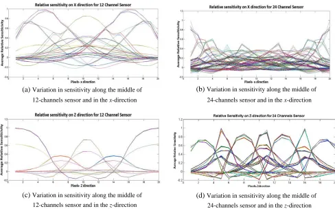
(a) Variation in sensitivity along the middle of 12-channels sensor and in the x-direction
(b) Variation in sensitivity along the middle of
24-channels sensor and in the x-direction
(c) Variation in sensitivity along the middle of 12-channels sensor and in the z-direction
(d) Variation in sensitivity along the middle of 24-channels sensor and in the z-direction
regions with both small slopes and amplitudes. The remaining of this paper will focus on describing experiments that confirm such predictions.
4. EXPERIMENTS AND DISCUSSION
Several experiments were carried out to compare the relative performances. An acquisition system with 24 channels from Tech4Imaging LLC was used with both sensors. For the sensor with 12 plates, only the first 12 channels of the acquisition box were used and the rest were blocked. The reconstruction algorithm employed was the 3D-NNMOIRT with identical iteration number and penalty coefficient [9, 15], and with the imaging domain divided into 203 = 8000 voxels (unknowns). By controlling every other possible variable, the quality of the reconstructed images is set mainly by the difference in the number of plates. Both sensors were built around cylinder columns made from acrylic. For each column, the height was 18 inches, inner diameter was 4 inches, and outer diameter was 4.5 inches, while the wall thickness was 0.25 inches. The imaging domain has 4.5 inches in diameter and 7.5 inches in height. The signal-to-noise ratio of the acquired data is inversely related to the acquisition speed. For higher acquisition speeds, less number of cycles is averaged for each capacitance reading, yielding a higher noise component in the final measurement. The data acquisition speed used in this study was 200 frames per second for the 12 channel sensor and 48 frames per second for the 24 channel sensor. To maintain consistency over for both sensors, the same 76 micro-second acquisition time was used for each capacitance data point. As the 24 channel sensor requires more capacitance data points to construct an imaging frame, the frame rates for both sensors were different. In any case, a detailed analysis of resolution limits versus signal-to-noise ratio and further larger number of electrodes is beyond the scope of this paper.
4.1. Simple Geometrical Objects
4.1.1. Single Sphere
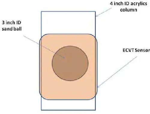
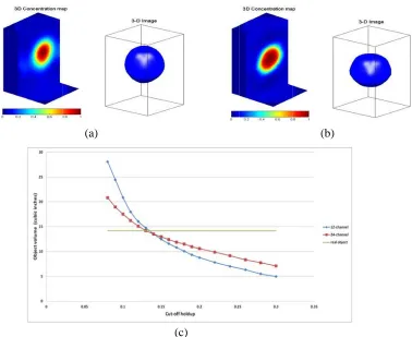
The first experiment was conducted considering a simple solid object inside the imaging domain, viz., a hollow plastic sphere stuffed with sand. The diameter of the sand ball was 3 inches and the thickness of the plastic shell around it was 0.03 inch. The ball was hung in the middle of the acrylic cylinder column by a very thin thread. Figure 6 illustrates the experimental setup. Figures 7(a) and 7(b) show the reconstructed images using the 12- and 24-channels sensors, respectively. The isosurface images
(a) (b)
(c)
Figure 7. Comparison of solid concentration as reconstructed by and 24-channels sensors. (a) 12-channels result. (b) 24-12-channels result. (c) Volume comparisons between both sensors results based on different cutoff values. Blue line is for 12 channels sensors and red line for 24 channel sensor.
in Figure 7 have a cut-off solids concentration of 0.21. From this figure, it is seen that both sensors can provide reasonable results for the material distribution, with the 24-channels sensor yielding better resolution. In particular, two distinct features are visible when using the 24-channels sensor. First, the image shape from 24-channels sensor better resembles that of a sphere when compared with the 12-channels result. The 12-channels image is distorted and resembles instead a water drop, having a noticeable distortion along the vertical direction. This can be explained by the fact that the 12-channels sensor has only three layers of plates whereas the 24-channels sensor has 4 layers, so the 24-channels sensor naturally has better vertical resolution. Second, we can also notice that the reconstructed permittivity gradients are different. For the 12-channels, the gradient near the surface is smaller than in the 24-channels sensor, leading to a ‘thick’ surface layer. A larger gradient exists inside the reconstructed sphere and the permittivity changes significantly near the center region inside the sand sphere. On the other hand, the 24-channels result shows a sharper change near the edge of the sphere and a relatively uniform distribution inside the sphere, which captures the real object better. An explanation for this difference is that in each layer there are 6 plates for the 24-channels sensor, so that both the horizontal and vertical resolutions are improved versus the 12-channels sensor. One can thus conclude that the 24-channels sensor shows a better performance in capturing both “edges” and gradients of dielectric distributions.
high-Figure 8. Experimental setup for imaging two spheres using ECVT sensors with 12 and 24 channels.
(a) (b)
Figure 9. Volumetric images of two spheres using 12- and 24-channel sensors. (a) 12 24-channel result. (b) 24 24-channel result.
permittivity object can be simply estimated as Vob = (m/M)V. In this experiment, for both sensors, M = 8000 and V = 14πD2H = 14π×4.52 ×8 = 127.2 inch3. The volume of the real sphere object is 14.14 inch3. Figure 7(c) shows the calculated volume comparisons from the two sensors and the real true volume under different cut-off holdups. The 0.21 cutoff was selected as it is close to where both sensors yield volume estimations closer to the actual sphere. It is clear that the 24-channel sensor has a better performance compared to 12-channel sensor, as the progression of error away from the optimal cutoff is considerably slower for the former.
To further compare the two sensors quantitatively, we also compute the mean-squared-error (MSE) of each reconstruction The MSE from each sensor is calculated using
MSE = 1 M
M
1 (Gi−Goi)
2 (1)
whereGi is the reconstructed (relative permittivity) value in voxel i, andGoi is the actual permittivity value at that voxel location (either inside or outside the sphere). The calculated MSE for the 12-channels sensor is 0.0544, while for the 24-channels is 0.0347. Although the estimated volume of the reconstructed spheres from both sensors is close, the MSE of 12-channels sensor is significantly higher than the MSE of the 24-channels sensor results because of the two factors noted before: higher sphericity and more uniform (accurate) permittivity distribution inside the reconstructed sphere.
4.1.2. Combination of Spheres
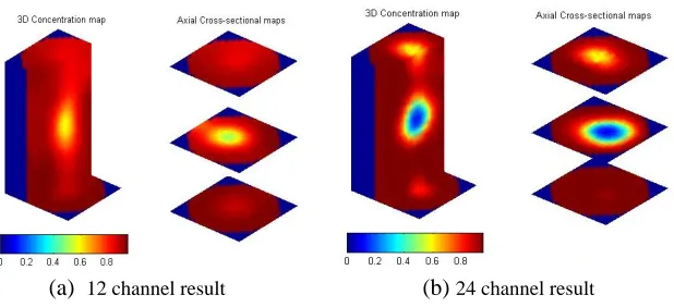
The next example consisted of two sand spheres of different sizes. The smaller sphere was the same used in the first experiment. The larger sphere was also a hollow plastic object stuffed with sand, but with a diameter of 4 inches. Inside the column, the smaller sphere was placed below the larger sphere, as shown in Figure 8.
Figure 10. Object used for testing 12 and 24 channels sensors.
(a) (b)
Figure 11. Reconstruction results of the complex object in Figure 10 using 12- and 24-channels sensors. (a) 12 channel result. (b) 24 channel result.
4.2. Composite-shaped Objects
The third experiment deals with an object of composite shape consisting of a square plate with a circular hole in its center, as shown in Figure 10. The object is made with clear-cast acrylic plastic board with thickness of 0.69 inches. The side length of square is 3 inches and the diameter of the inner round hole is 2 inches. Similar to the first experiment, the object is hung in the middle of the acrylics cylinder column by a very thin thread. Figure 11 shows the reconstruction results using 12- and 24-channels sensors. Similar to Figure 9, one observes that the image quality from the 24-channels sensor is clearly superior because the image of the 12-channel sensor fails to capture the correct shape, while for the 24-channel sensor the square shape is better reproduced and the dimensions of the reconstructed object are closer to the original object. In addition, the round hole in the center of the plate can also be distinguished. An observation should be made here about the dielectric distribution values, as the 24-channels sensor estimates a maximum value significantly less than 1. This is simply because the sensors were calibrated with sand which has a dielectric constant close to 10, whereas the experiment was conducted with acrylic plastic having a dielectric constant close to 2. The authors elected to conduct this experiment with the sand calibration to demonstrate that the system can resolve the dielectric distribution, even when calibrated with a material of higher dielectric constant. This is especially important as most of ECVT application relate to multiphase flow systems. In multiphase flows, the dielectric distribution changes based on changes in the material phase holdup (i.e., proportion of solids to gas, for example). In cases where the flow is dilute (i.e., solids concentration with respect to gas is low), it is critical to be able to reconstruct the phase concentration for better understanding of the observed flow process.
4.3. Gas-Solid Fluidization System
Figure 12. Experimental-setup for imaging FCC fluidized bed with 12- and 24-channels sensors.
(a) 12 channel result (b) 24 channel result
Figure 13. Results of (a) 12 and (b) 24 channels sensors for imaging FCC bubbling bed.
blown upward from the gas distributor as the fluidization gas. Figure 12 depicts the experimental setup employed for testing both sensors.
(a) (b)
Figure 14. Radial profiles of solids concentration for (a) 12 channels sensor and (b) 24 channel sensor corresponding to results in Figure 13.
Figure 15. Experimental setup of the gas-liquid bubbling system used to test the 12- and 24-channels sensors.
(a) 12 channel result (b) 24 channel result
4.4. Gas-Liquid System
Gas-liquid bubble columns are widely used in the chemical industry. Similar to the gas-solid fluidization system, air was used as the gas phase. Mineral spirit was chosen as the liquid phase because of its low relative permittivity and insulation property, as well as its good fluidity. A 0.75 inch diameter nozzle was used as the gas distributor. Figure 15 shows the experimental setup and Figure 16 shows results from both sensors under similar superficial gas velocity (0.1 ft/s), where we can see that the 24-channels sensor image has more details compared to the 12-channels image. The center of the bubble is correctly reconstructed with near zero liquid concentration (i.e., “empty”) in the 24-channels sensor result, which is not the case in 12-channels image. This result is in accord with fluid mechanics predictions that a rising bubble in a viscous liquid should contain close to zero liquid concentration [19].
5. CONCLUDING REMARKS
We compared the performance of two ECVT sensors with 12- and 24-channels respectively, in a variety of experimental conditions. Experiments involving simple static objects, a composite-shape static object, a gas-solids fluidized bed, and a gas-liquid bubbling system were considered for comparison. The use of such controlled experiments allowed to better evaluate and compare the two systems, and to assess the impact of different parameters on the sensor performance. Variables that can affect the image quality were controlled so that the relative difference in performance (resolution) can be attributed primarily to the increase in number of channels. In particular, the same reconstruction algorithm was employed (with same choice of parameters) and both sensors were designed with similar plate shapes covering an equal volume. Results from all experiments indicated that increasing the total number of channels from 12 to 24 provides a marked increase on ECVT image resolution. These conclusions are expected to translate to practical scenarios where the variables, here under control, can vary simultaneously with combined effects that reproduce the observed trends. Finally, we note that the use of an even larger number of channels, beyond 24, is also of interest. Such exploitation of very large number of channels is of particular relevance to both adaptive [20, 21] and dual modality [22, 23] ECVT systems, for enhancing information acquisition.
ACKNOWLEDGMENT
This work has been supported by the US Department of Energy (DOE). The published material represents the position of the author(s) and not necessarily that of the DOE. Funding for Open Access provided by The Ohio State University Open Access Fund.
REFERENCES
1. Wang, H. and W. Yang, “Scale-up of an electrical capacitance tomography sensor for imaging pharmaceutical fluidized beds and validation by computational fluid dynamics,” Meas. Sci. Technol., Vol. 22, No. 10, 104015, 2011.
2. Yang, D. Y., B. Zhou, C. L. Xu, and S. M. Wang, “Thick-wall electrical capacitance tomography and its application in dense-phase pneumatic conveying under high pressure,” IET Image Proc., Vol. 5, No. 5, 513–522, 2011.
3. Rimpil¨ainen, V., S. Poutiainen, L. M. Heikkinen, T. Savolainen, M. Vauhkonen, and J. Ketolainen, “Electrical capacitance tomography as a monitoring tool for high-shear mixing and granulation,” Chem. Eng. Sci., Vol. 66, No. 18, 4090–4100, 2011.
4. Chandrasekera, T. C., A. Wang, D. J. Holland, Q. Marashdeh, M. Pore, F. Wang, A. J. Sederman, L. S. Fan, L. F. Gladden, and J. S. Dennis, “A comparison of magnetic resonance imaging and electrical capacitance tomography: An air jet through a bed of particles,” Powder Technol., Vol. 227, 86–95, 2012.
in a gas-solid fluidised bed,”Particuology, Vol. 10, 161–169, 2012.
9. Marashdeh, Q., W. Warsito, L.-S. Fan, and F. L. Teixeira, “Non-linear image reconstruction technique for ECT using a combined neural network approach,” Meas. Sci. Technol., Vol. 17, No. 8, 2097–2103, 2006.
10. Soleimani, M., P. K. Yalavarthy, and H. Dehghani, “Helmholtz-type regularization method for permittivity reconstruction using experimental phantom data of electrical capacitance tomography,”IEEE Tran. Instr. Meas., Vol. 59, No. 1, 78–83, 2010.
11. Lei, J., S. Liu, H. H. Guo, Z. H. Li, J. T. Li, and Z. X. Han, “An image reconstruction algorithm based on the semiparametric model for electrical capacitance tomography,” Comp. Math. Appl., Vol. 61, No. 9, 2843–2853, 2011.
12. Cao, Z., L. Xu, and H. Wang, “Image reconstruction technique of electrical capacitance tomography for low-contrast dielectrics using Calderon’s method,”Meas. Sci. Technol., Vol. 20, No. 10, 2009. 13. Yang, W., “Design of electrical capacitance tomography sensors,” Meas. Sci. Technol., Vol. 21,
No. 4, 042001, 2010.
14. Peng, L., J. Ye, G. Lu, and W. Yang, “Evaluation of effect of number of electrodes in ECT sensors on image quality,”IEEE Sensors J., Vol. 12, No. 5, 1554–1565, 2012.
15. Warsito, W. and L. S. Fan, “Neural network multi-criteria optimization image reconstruction technique (NN-MOIRT) for linear and non-linear process tomography,”Chem. Eng. Proc., Vol. 42, 663–674, 2003.
16. Marashdeh, Q. and F. L. Teixeira, “Sensitivity matrix calculation for fast electrical capacitance tomography (ECT) of flow systems,”IEEE Trans. Magn., Vol. 40, No. 2, 1204–1207, 2004. 17. Marashdeh, Q., W. Warsito, L.-S. Fan, and F. L. Teixeira, “Nonlinear forward problem solution
for electrical capacitance tomography using feed forward neural network,”IEEE Sensors J., Vol. 6, No. 2, 441–449, 2006.
18. Yates, J. G., D. J. Cheesman, and Y. A. Sergeev, “Experimental observations of voidage distribution around bubbles in a fluidized bed,”Chem. Eng. Sci., Vol. 49, 1885–1895, 1994.
19. Bhaga, D. and M. E. Weber, “Bubbles in viscous liquids: Shapes, wakes and velocities,” J. Fluid Mech., Vol. 105, 61–85, 1981.
20. Marashdeh, Q. M., F. L. Teixeira, and L.-S. Fan, “Adaptive electrical capacitance volume tomography,”IEEE Sensors J., Vol. 14, No. 4, 1253–1259, 2014.
21. Zeeshan, F., L. Teixeira, and Q. Marashdeh, “Sensitivity map computation in adaptive electrical capacitance volume tomography with multielectrode excitations,” Electron. Lett., Vol. 51, No. 4, 334–336, 2015.
22. Marashdeh, Q., W. Warsito, L.-S. Fan, and F. L. Teixeira, “A multimodal tomography system based on ECT sensors,”IEEE Sensors J., Vol. 7, No. 3, 426–433, 2007.