Diffraction by a Dielectric Wedge on a Ground Plane
Marcello Frongillo1, Gianluca Gennarelli2, and Giovanni Riccio3, *
Abstract—The plane wave diffraction by an acute-angled wedge located on a perfect electric conducting plane is studied in the frequency and time domains. Only a TMz polarization is explicitly considered in the manuscript since the case of a TEz polarization can be solved in a similar way. At first, the uniform asymptotic physical optics approach is used to obtain the diffraction coefficients in the framework of the uniform geometrical theory of diffraction. The analytical procedure allows one to obtain closed form expressions that are easy to handle and provide reliable results from the engineering viewpoint. The time domain diffraction coefficients are successively determined by applying the inverse Laplace transform to the frequency domain counterparts. The effectiveness of the proposed solutions is proved by means of numerical tests and comparisons with full-wave numerical techniques.
1. INTRODUCTION
Electromagnetic engineers working in many application areas appreciate the availability of tools based on the Uniform Geometrical Theory of Diffraction (UTD) [1] since it provides a simple physical representation of the wave propagation in terms of incident, reflected, transmitted, and diffracted rays. On the other hand, numerical techniques give no physical meanings and require a large amount of time and computing resources at high frequencies.
The frequency domain Uniform Asymptotic Physical Optics (FD-UAPO) approach has recently emerged as a useful and alternative high-frequency method to obtain closed form approximate solutions to plane wave diffraction problems [2]. No special functions and integral equations must be computed by means of numerical techniques since such solutions contain the UTD transition function and the Geometrical Optics (GO) response of the structure in terms of reflection and transmission coefficients. The FD-UAPO solutions result from an analytic procedure and are easy to handle in the UTD context. They compensate the GO field discontinuities and their accuracy has been tested using available numerical tools. Note that they produce inaccuracies in specific well-known cases (e.g., grazing incidence with respect to the illuminated surface of the structure) since they are based on the PO approximation. Two-dimensional problems of plane wave diffraction by isolated dielectric wedges have been solved by means of the FD-UAPO approach [3–6] by dividing the observation domain into two parts: the wedge shaped (internal) region and the surrounding free space. The ray-tracing technique has been used to determine the GO field accounting for the multiple reflection and transmission propagation mechanisms generated by the wedge geometry. In particular, the knowledge of the GO field at the internal and external planar faces of the dielectric has permitted to calculate the electric and magnetic equivalent PO surface currents. The scattering problem in the external (internal) sub-domain has been tackled considering the equivalent PO surface currents on the external (internal) faces of the wedge as sources in the radiation integral that has been reduced to a standard form by using useful approximations and analytic evaluations. The Steepest Descent Method and the Multiplicative Method
Received 6 March 2019, Accepted 31 May 2019, Scheduled 16 June 2019
* Corresponding author: Giovanni Riccio ([email protected]).
have been successively applied to extract the diffraction contribution associated to each face. Numerical tests have demonstrated the effectiveness of the corresponding FD-UAPO solutions for the diffraction coefficients to be used in the UTD framework.
It is worth noting that the diffraction by penetrable wedges is a challenging problem from the analytic viewpoint. Some existing methods provide analytical and heuristic approximate solutions under certain assumptions, others try to solve the problem in an exact sense combining analytical and numerical techniques that often limit the computation efficiency and applicability of the approach. Representative results in the frequency domain can be found in [7–19].
The UTD-like formulation of the FD-UAPO diffraction coefficients for the problems tackled in [3– 6] has permitted to determine the time domain (TD) counterparts in closed form according to [20]. The inverse Laplace transform has been applied under the hypothesis that the dielectric parameters are independent of the frequency. The corresponding TD-UAPO diffraction coefficients have been presented in [6, 21–23] and used to evaluate the transient diffracted field originated by an arbitrary function plane wave via a convolution integral.
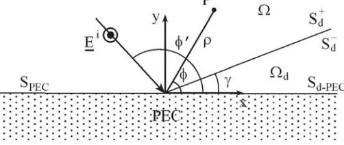
The goal of this manuscript is to propose the FD- and TD-UAPO diffraction coefficients associated with a TMz plane wave impacting a composite structure formed by a tapered infinite dielectric wedge on a perfect electric conducting (PEC) half-space (see Fig. 1). The FD-UAPO diffraction coefficients relevant to a TEz plane wave into the free-space and dielectric regions can be determined accounting for the results presented in [3–5]. In particular, the TEz diffraction coefficients differ by a “—” sign from the TMz ones under the condition to use the reflection and transmission coefficients for the parallel polarization instead of those associated to the perpendicular polarization. The FD- and TD-UAPO diffraction coefficients for a structure composed by metallic and dielectric 90◦ blocks have been recently proposed by the authors [24].
The incidence direction is orthogonal to the dielectric edge, so that a two-dimensional problem is tackled. The ray-tracing analysis and the GO field evaluation into the free-space and dielectric regions are reported in Section 2. The successive section is dedicated to the FD-UAPO solutions that are validated by means of numerical tests and comparisons with FDTD data, whereas the TD-UAPO counterparts are presented in Section 4. Conclusions are presented in Section 5.
2. THE GO FIELD
The two-dimensional geometry of the considered problem is depicted in Fig. 1. A dielectric wedge with internal apex angle γ < π/2 is positioned upon a PEC half-space and its edge coincides with the z axis of a Cartesian coordinates system having they axis perpendicular to the PEC surface. The wedge sector is indicated by Ωd and is filled by a lossless non-magnetic medium characterized by the relative permittivity εr. The composite structure is surrounded by the free-space region Ω with impedanceζ0
and propagation constant k0. The electric field associated to a TMz plane wave from Ω is expressed
by Ei =E0ie−jk0·rzˆ, wherek0 =k0(−cosφxˆ−sinφyˆ) and r =ρ(cosφxˆ+ sinφyˆ) denotes the position
vector of the observation point P.
This Section is devoted to the evaluation of the GO field that will be used in the next section to
compute the PO surface currents involved in the FD-UAPO approach.
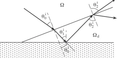
The incident wave is reflected by SP EC and Sd in Ω and transmitted into Ωd according to the Snell’s laws. Unfortunately the previous statement does not fully describe the GO field propagation in the observation regions since the transmitted wave into Ωdoriginates a bouncing wave (see Fig. 2) that generates further GO contributions in Ω until the total reflection occurs within the wedge. Note that if γ < φ < γ+π/2 the bouncing wave propagates initially toward the edge and successively away from it [6]. In addition, ifπ−γ < φ < πthe complexity of the wave propagation analysis increases because of a second incident wave that illuminates Sd after the reflection by SP EC. This additional incident wave produces further GO contributions that can be independently determined and added to those due to the main incident wave. According to the previous statements, a growth in complexity occurs if γ < φ < γ+π/2 orπ−γ < φ < π without adding more information about the method proposed to solve the diffraction problem, and therefore the direction γ+π/2< φ < π−γ is chosen from this point on to determine the GO field and the FD-UAPO diffracted field.
Figure 2. Ray tracing.
The ray-tracing scheme relevant to the considered case is shown in Fig. 2. The incident wave penetrates into Ωd with transmission angle θ0t = sin−1(sinθ0i/
√
εr), where θi0 = φ −(γ +π/2), and
propagates toward Sd−P EC with incidence directionθ1i =θ0t+γ. The wave is then reflected bySd−P EC and propagates toward Sd, where it is successively reflected with direction θr2 = θ2i = θ0t + 2γ and
transmitted into Ω with transmission angle θt2 = sin−1(
√
εrsinθ2i). Such a propagation scheme is
iterated untilθnr =θni =θ0t+nγ < π/2−γ and produces transmission contributions in Ω until the total
reflection occurs inside the wedge, i.e., when θi
n> θc = sin−1(1/√εr). Accordingly, the GO field at any point of the observation regions can be evaluated by means of the following expressions:
EGOΩ (P) =
ejk0ρcos(φ−φ)−
ejk0ρcos(φ+φ)
U(φ−φRBP EC) + Γ0e
jk0ρcos((φ−γ)+(φ−γ))
U(φRBd−φ)
+T0
⎡ ⎢ ⎣
N
n=1
n even Tn
n−1
m=1
Γm e−jk0ρsin((φ−γ)+θt n)Uθ
c−θni
U
π
2−θ t
n−(φ−γ)
⎤⎥ ⎦
⎫ ⎪ ⎬ ⎪ ⎭E
i
0zˆ(1)
EGOΩd(P) = ⎧ ⎪ ⎨ ⎪ ⎩e
jkdρsin((φ−γ)−θt0) +
N
n=1
n even
n
m=1
Γm ejkdρsin((φ−γ)−θin)
+ N
n=1
n odd
n
m=1
Γm e−jkdρsin((φ−γ)+θni+1)
⎫ ⎪ ⎬ ⎪ ⎭T0E
i
0zˆ (2)
whereU(θ) = 1 ifθ >0 or U(θ) = 0 otherwise, N = Int[(π/2−θt
0)/γ], with Int[·] denoting the integer
part of the argument, kd = k0√εr is the propagation constant of the dielectric, φRBP EC = π −φ
θtn= sin−1(√εrsinθin) is the transmission angle at then-th step,
Γ0 =
cosθi0− √εrcosθ0t
cosθi
0+
√
εrcosθ0t
(3)
T0 =
2 cosθ0i
cosθi0+
√
εrcosθ0t
(4)
Γm = √
εrcosθim−cosθtm √
εrcosθi
m+ cosθtm
ifm is even or Γm=−1 ifm is odd (5)
Tn =
2√εrcosθni √
εrcosθin+ cosθnt
(6)
3. THE FD-UAPO DIFFRACTED FIELD
Two distinct problems relevant to the dielectric region and the surrounding space are tackled. For each of them, the knowledge of the GO field on the surfaces bounding the region allows one to evaluate the electric (Js) and magnetic (Jms) equivalent PO surface currents to be used as sources on the dielectric surfaces.
3.1. Free-Space Region Ω
The radiation integral is considered to determine the scattered field due to sources onSd+∪SP EC:
EsΩ = −jk0
Sd+
I−RˆRˆ
ζ0(Js)S+
d + (Jms)Sd+×
ˆ R
e−jk0R 4πR dS
+
d
−jk0
SP EC
I−RˆRˆ
ζ0(Js)SP EC
e−jk0R
4πR dSP EC (7)
where I denotes the identity matrix; ˆR is the unit vector from the source point S(r(ρ, z)) to P; R=|r−r(ρ, z)|is the corresponding distance, and
ζ0(Js)SP EC = 2E0isinφejk0ρ
cos(π−φ)
ˆ
z (8)
ζ0(Js)S+
d = ⎡ ⎢
⎣(1−Γ0) sin(φ−γ)ejk0ρ
cos(φ−γ)
−T0
N
n=1
n even Tn
n−1
m=1
Γm cosθtne−jk0ρsinθt nUθ
c−θni
⎤ ⎥ ⎦E0izˆ
(9)
(Jms)S+
d = ⎡ ⎢
⎣(1 + Γ0)ejk0ρ
cos(φ−γ)
+T0
N
n=1
n even Tn
n−1
m=1
Γm e−jk0ρsinθt nUθ
c−θni
⎤ ⎥
⎦E0i(−cosγxˆ−sinγyˆ)
(10) According to [2], the next step is the use of the unit vector of the diffraction direction ˆs = cosφxˆ+ sinφyˆinstead of ˆR in Eq. (7):
EsΩ = −
jk0
4π
(1−Γ0) sin(φ−γ) +∞ 0 +∞ −∞
ejk0ρcos(φ−γ)e−jk0|r−r
(ρ,z)|
|r−r(ρ, z)|dz
dρ
−T0
N
n=1
n even Tn
n−1
m=1
Γm cosθntUθc−θni
+∞ 0 +∞ −∞
ejk0ρcos(θtn+π/2)e
−jk0|r−r(ρ,z)|
|r−r(ρ, z)|dz
−(1 + Γ0) sin(φ−γ) +∞
0 +∞
−∞
ejk0ρcos(φ−γ)e−jk0|r−r
(ρ,z)|
|r−r(ρ, z)|dz
dρ
−T0sin(φ−γ)
N
n=1
n even Tn
n−1
m=1
Γm Uθc−θni
+∞
0 +∞
−∞
ejk0ρcos(θt n+π/2)e
−jk0|r−r(ρ,z)|
|r−r(ρ, z)|dz
dρ
+2 sinφ
+∞
0 +∞
−∞
ejk0ρcos(π−φ)e−jk0|r−r
(ρ,z)|
|r−r(ρ, z)| dz
dρEi
0zˆ (11)
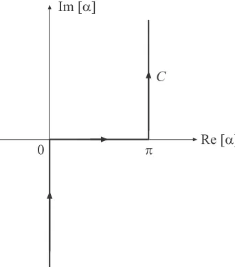
since (I−sˆˆs)ˆz= ˆz. The integration along z provides the zeroth order Hankel function of the second kind that can be expressed by using a useful integral representation [25]. The Sommerfeld-Maliuzhinets inversion formula [26] is successively applied, thus obtaining the following result:
−jk0
4π
+∞
0 +∞
−∞
ejk0ρcosξ(φ)e−jk0|r−r
(ρ,z)|
|r−r(ρ, z)|dz
dρ = 1
j4π
C
e−jk0ρcos(α−ξ(φ))
cosα+ cosξ(φ)dα (12)
where C is the integration path in the complex α-plane shown in Fig. 3. The integral in Eq. (12) is reduced to a typical diffraction integral that is evaluated by means of the Steepest Descent Method and the Multiplicative Method in the high-frequency approximation [2].
Re [α] Im [α]
C
0 π
Figure 3. The integration pathC in the complexα-plane.
At the end of the analytical procedure that is previously summarized, the diffracted field contribution associated to Eq. (11) is expressed by:
EdΩ = (1−Γ0) sin(φ−γ)−(1 + Γ0) sin(φ−γ)
Ft
2k0ρcos2(((φ−γ) + (φ−γ))/2)
cos(φ−γ) + cos(φ−γ)
−T0
N
n=1
n even Tn
⎛ ⎜ ⎝
n−1
m=1
m even Γm
⎞ ⎟
⎠(−1)n/2sin(φ−γ) + cosθtnU(θC−θni)
×Ft
2k0ρcos2
(φ−γ) + (θt
n+π/2)
/2 cos(φ−γ) + cos(θt
+2 sinφFt
2k0ρcos2(((π−φ) + (π−φ))/2)
cos(π−φ) + cos(π−φ)
e−jπ/4 2√2πk0
e−jk0ρ √
ρ E i
0zˆ=DΩe −jk0ρ
√ ρ E
i
0ˆz (13)
where Ft(·) is the standard UTD transition function [1]. Accordingly, the FD-UAPO diffraction coefficientDΩ is expressed in closed form and contains standard parameters and functions.
3.2. Dielectric Region Ωd
The PO surface currents on Sd−∪Sd−P EC are used as sources to solve the internal scattering problem. The analytical procedure previously presented to evaluate DΩ is now applied to determine DΩd, thus
obtaining:
DdΩ = T0 sin(φ−γ)−cos(θ0t)
Ft
2kdρcos2
(2π−φ+γ) + (θt
0+π/2)
/2 cos(φ−γ) + cos(θt0+π/2)
+ N
n=1
n even
⎛ ⎜ ⎝
n−1
m=1
m even Γm
⎞ ⎟
⎠(−1)n/2(1 + Γn) sin(φ−γ) + (1−Γn) cosθni
×Ft
2kdρcos2
(φ−γ) + (θni +π/2)/2 cos(φ−γ) + cos(θi
n+π/2)
+ N
n=1
n odd
⎛ ⎜ ⎝
n−1
m=1
m even Γm
⎞ ⎟
⎠(−1)(n−1)/2cosθni Ft
2kdρcos2(φ−2π)+(θin+π/2)/2 cosφ+ cos(θi
n+π/2)
e−jπ/4 2√2πkd
(14)
Accordingly, the corresponding diffracted field is:
EdΩd =DΩd
e−jkdρ
√ ρ E
i
0zˆ (15)
3.3. Numerical Tests
This part is devoted to show the results of some numerical tests to prove the efficiency and the accuracy of the proposed solutions.
0 20 40 60 80 100 120 140 160 180
0
0 20 40 60 80 100 120 140 160 180 0
Figure 5. Total field whenεr = 2,γ = 15◦,φ= 120◦,ρ= 5λ0.
30 60 90
120
150
180
210
240
270 300 330 -60 -40 -20 0
PEC
UAPO-based approach FDTD
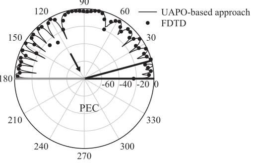
Figure 6. Data comparison whenεr= 2, γ = 15◦,φ = 120◦,ρ= 5λ0.
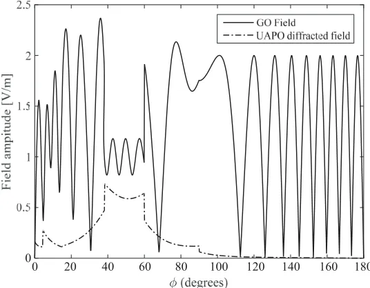
The first set of figures refers to a wedge that is characterized byεr = 2 andγ = 15◦. The structure is lit by an incident plane wave at φ = 120◦ and P moves on a circular path with ρ = 5λ0, where
λ0 is the free-space wavelength. According to the input data, the GO field possesses four boundaries
corresponding (from left to right in Fig. 4) to the internal reflections (φ∼= 5◦), transmission through Sd (φ ∼= 38◦), reflection by SP EC (φ = 60◦) and reflection by Sd (φ = 90◦). The UAPO diffracted field is reported in Fig. 4 and permits to obtain a total field that is continuous over the full path (see Fig. 5), thus confirming that its contribution is able to compensate the discontinuities of the GO field. The accuracy of the solutions has been tested by means of a FDTD code that implements the total field/scattered field technique [27]. A normalized dB scale is adopted in the next figures to compare the data. Fig. 6 shows the results for the considered case and makes evident a good agreement between the data. It is important to remember that the UAPO solutions result from more than one approximation in the analytical procedure.
30 60 90
120
150
180
210
240
270 300 330 -60 -40 -20 0
PEC
UAPO-based approach FDTD
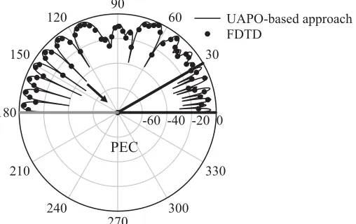
Figure 7. Data comparison whenεr= 5, γ = 30◦,φ = 135◦,ρ= 5λ0.
30 60 90
120
150
180
210
240
270 300 330 -60 -40 -20 0
PEC
UAPO-based approach FDTD
Figure 8. Data comparison whenεr= 10, γ = 30◦,φ = 135◦,ρ= 5λ0.
4. THE TD-UAPO DIFFRACTED FIELD
The TD counterparts of Eqs. (13) and (15) are determined by using the following convolution integral:
edΩ,Ωd(P, t) = ˆz
1 √ ρ
t−ρ/c
t0
dΩ,Ωd
t−ρ c −τ
ei(Q, τ) dτ (16)
with t−ρ/c > t0. The forcing function is the incident field ei at the diffraction point Q, and c is the
speed of light in the considered observation region. The TD-UAPO diffraction coefficients dto be used in Eq. (16) are obtained by applying the inverse Laplace transform toD under the assumption thatεr is independent of the frequency. According to [20], their expressions are:
dΩ =
1 2√2π
⎧ ⎪ ⎪ ⎨ ⎪ ⎪ ⎩
(1−Γ0) sin(φ−γ)−(1 + Γ0) sin(φ−γ)
G
%
2ρcos2
%
(φ−γ) + (φ−γ) 2
&
, t
&
cos(φ−γ) + cos(φ−γ)
−T0
N
n=1
n even
(−1)n/2Tn
⎛ ⎜ ⎝
n−1
m=1
m even Γm
⎞ ⎟
× G
%
2ρcos2
%
(φ−γ) + (θtn+π/2) 2
&
, t
&
cos(φ−γ) + cos(θt
n+π/2)
U(θc−θni)
⎫ ⎪ ⎪ ⎬ ⎪ ⎪ ⎭
+sinφ
√ 2π
G
%
2ρcos2
% (π−φ) + (π−φ) 2 & , t &
cos(π−φ) + cos(π−φ) (17)
dΩd = T0
2√2π
⎧ ⎪ ⎪ ⎨ ⎪ ⎪ ⎩
sin(φ−γ)−cosθt0
G %
2ρcos2
%
(2π−φ+γ) + (θt0+π/2)
2
&
, t
&
cos(φ−γ) + cos(θ0t+π/2)
+ N
n=1
n even
(−1)n/2
⎛ ⎝ n−1
m=1
m even Γm
⎞
⎠ (1 + Γn) sin(φ−γ) + (1−Γn) cosθin
×G
%
2ρcos2
%
(2π−φ+γ) + (θin+π/2) 2
&
, t
&
cos(φ−γ) + cos(θi
n+π/2)
⎫ ⎪ ⎪ ⎬ ⎪ ⎪ ⎭
+√T0 2π
N
n=1
n odd
(−1)(n−1)/2
⎛ ⎝ n−1
m=1
m even Γm
⎞ ⎠cosθni
G
%
2ρcos2
%
(φ−2π) + (θi
n+π/2) 2
&
, t
&
cosφ+ cos(θi
n+π/2)
(18)
where
G(X, t) = √ X
π ct(t+X/c) (19)
5. CONCLUSIONS
Useful solutions have been proposed to evaluate the plane wave diffracted field in the free space surrounding the considered structure, as well as within the wedge-shaped dielectric. The UAPO approach in the frequency domain has been initially applied, and closed form expressions have been obtained for the diffraction coefficients. The corresponding field contributions are able to compensate all the GO field discontinuities inside and outside the dielectric, and guarantee a quite accurate total field. As a matter of fact, the FD-UAPO solutions suffer from PO approximation and do not account for the surface waves. Accordingly, such solutions represent a possible good choice if quite accurate results must be achieved by using UTD-like formulas. Moreover, TD-UAPO diffraction coefficients have been obtained by applying the inverse Laplace transform to the FD-UAPO counterparts. To the authors’ knowledge, no other closed form expressions are available in the time domain.
REFERENCES
1. Kouyoumjian, R. G. and P. H. Pathak, “A uniform geometrical theory of diffraction for an edge in a perfectly conducting surface,” Proc. IEEE, Vol. 62, 1448–1461, 1974.
2. Riccio, G., “Uniform asymptotic physical optics solutions for a set of diffraction problems,” Wave Propagation in Materials for Modern Applications, 33–54, A. Petrin Ed., Intech, Vukovar, HR, 2010.
3. Gennarelli, G. and G. Riccio, “A uniform asymptotic solution for diffraction by a right-angled dielectric wedge,”IEEE Trans. Antennas Propagat., Vol. 59, 898–903, 2011.
4. Gennarelli, G. and G. Riccio, “Plane-wave diffraction by an obtuse-angled dielectric wedge,” J. Opt. Soc. Am. A, Vol. 28, 627–632, 2011.
6. Frongillo, M., G. Gennarelli, and G. Riccio, “Plane wave diffraction by arbitrary-angled lossless wedges: High-frequency and time-domain solutions,” IEEE Trans. Antennas Propagat., Vol. 66, 6646–6653, 2018.
7. Berntsen, S., “Diffraction of an electric polarized wave by a dielectric wedge,”SIAM J. Appl. Math., Vol. 43, 186–211, 1983.
8. Rawlins, A. D., “Diffraction by, or diffusion into, a penetrable wedge,” Proc. R. Soc. Lond. A, Vol. 455, 2655–2686, 1999.
9. Burge, R. E., et al., “Microwave scattering from dielectric wedges with planar surfaces: A diffraction coefficient based on a physical optics version of GTD,”IEEE Trans. Antennas Propagat., Vol. 47, 1515–1527, 1999.
10. Rouviere, J. F., N. Douchin, and P. F. Combes, “Diffraction by lossy dielectric wedges using both heuristic UTD formulations and FDTD,” IEEE Trans. Antennas Propagat., Vol. 47, 1702–1708, 1999.
11. Seo, C. H. and J. W. Ra, “Plane wave scattering by a lossy dielectric wedge,” Microwave Opt. Technol. Lett., Vol. 25, 360–363, 2000.
12. Kim, S. Y., J. W. Ra, and S. Y. Shin, “Diffraction by an arbitrary-angled dielectric wedge: part I — Physical optics approximation,” IEEE Trans. Antennas Propagat., Vol. 39, 1272–1281, 1991. 13. Kim, S. Y., J. W. Ra, and S. Y. Shin, “Diffraction by an arbitrary-angled dielectric wedge. II.
Correction to physical optics solution,” IEEE Trans. Antennas Propagat., Vol. 39, 1282–1292, 1991.
14. Bernardi, P., R. Cicchetti, and O. Testa, “A three-dimensional UTD heuristic diffraction coefficient for complex penetrable wedges,”IEEE Trans. Antennas Propagat., Vol. 50, 217–224, 2002.
15. Salem, M. A., A. H. Kamel, and A. V. Osipov, “Electromagnetic fields in presence of an infinite dielectric wedge,”Proc. R. Soc. Lond. A, Vol. 462, 2503–2522, 2006.
16. Daniele, V. and G. Lombardi, “The Wiener-Hopf solution of the isotropic penetrable wedge problem: Diffraction and total field,”IEEE Trans. Antennas Propagat., Vol. 59, 3797–3818, 2011. 17. Vasilev, E. N. and V. V. Solodukhov, “Diffraction of electromagnetic waves by a dielectric wedge,”
Radiophysics and Quantum Electronics, Vol. 17, 1161–1169, 1976.
18. Vasil´ev, E. N., V. V. Solodukhov, and A. I. Fedorenko, “The integral equation method in the problem of electromagnetic waves diffraction by complex bodies,” Electromagnetics, Vol. 11, 161– 182, 1991.
19. Budaev, B., Diffraction by Wedges, London, Longman Scient, 1995.
20. Veruttipong, T. W., “Time domain version of the uniform GTD,”IEEE Trans. Antennas Propagat., Vol. 38, 1757–1764, 1990.
21. Gennarelli, G. and G. Riccio, “Time domain diffraction by a right-angled penetrable wedge,”IEEE Trans. Antennas Propagat., Vol. 60, 2829–2833, 2012.
22. Gennarelli, G. and G. Riccio, “Obtuse-angled penetrable wedges: A time domain solution for the diffraction coefficients,” Journal of Electromagnetic Waves and Applications, Vol. 27, No. 16, 2020–2028, 2013.
23. Frongillo, M., G. Gennarelli, and G. Riccio, “TD-UAPO diffracted field evaluation for penetrable wedges with acute apex angle,” J. Opt. Soc. Am. A, Vol. 32, 1271–1275, 2015.
24. Frongillo, M., G. Gennarelli, and G. Riccio, “Diffraction by a structure composed of metallic and dielectric 90◦ blocks,”IEEE Antennas Wireless Propagat. Lett., Vol. 17, 881–885, 2018.
25. Clemmow, P. C., The Plane Wave Spectrum Representation of Electromagnetic Fields, Oxford, Oxford University Press, 1996.
26. Maliuzhinets, G. D., “Inversion formula for the Sommerfeld integral,” Soviet Physics Doklady, Vol. 3, 52–56, 1958.