Analysis of Co-Channel Interference at Waveguide Joints Using Multiple Cavity Modeling Technique

(1)

ANALYSIS OF CO-CHANNEL INTERFERENCE AT WAVEGUIDE JOINTS USING MULTIPLE CAVITY MODELING TECHNIQUE

D. K. Panda and A. Chakraborty

Department of Electronics and Electrical Communication Engineering Indian Institute Of Technology

Kharagpur, West Bengal, 721302, India

S. R. Choudhury

Department of Electronics Communication Engineering and Electronics Instrumentation Engineering

College of Engineering and Management Kolaghat Mecheda, Midnapur (E), WB, 721171, India

Abstract—A method of moment based analysis of the co-channel interference at waveguide joints has been presented using Multi Cavity Modeling Technique (MCMT). The proposed analysis has good agreement with the theoretical; CST microwave studio and HFSS simulated data.

1. INTRODUCTION

Low cost, low profile two dimensional scanning phased array antennas have wide application in Low Earth Orbit (LEO), Middle Earth Orbit (MEO) and Geostationary Earth Orbit (GEO) satellite communication. Multi-port Power divider has already found wide applications in phased array techniques. At the input of the two dimensional array mainly longitudinal power dividers are in use. Due to faulty workman-ship there may be a gap at the flange joints which causes the power coupling to the neighbor ports. However the problems of theoretical analysis of this power coupling remains unsolved. Effort has been made to model this interference using a regular structure with adding a uniform gap at the joints.

(2)

92 Panda, Chakraborty, and Choudhury

Technique (MCMT) [1]. The technique involves in replacing all the apertures and discontinuities of the waveguide structures, with equivalent magnetic current densities so that the given structure can be analyzed using only Magnetic Field Integral Equation (MFIE). Since only the magnetic currents present in the apertures are considered the methodology involves only solving simple magnetic integral equation rather than the complex integral equation involving both the electric and magnetic current densities.

2. FORMULATION OF THEORY

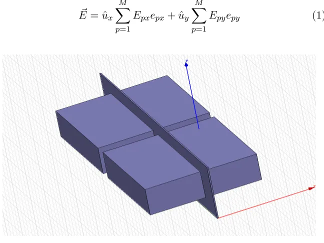
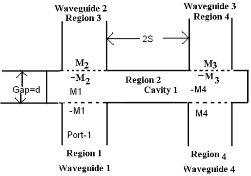
The diagram of a basic flange with two waveguide sections connected with another one with finite gap is shown in Fig. 1and its cavity modeling and details of region is shown in Fig. 2 which shows that the structures have 4 waveguide regions and 1cavity region. For the cavity modeling purposes a uniform gap is assumed and also the boundaries are covered with electric conductors. The interfacing apertures between different regions are replaced by equivalent magnetic current densities. The electric field at the aperture is assumed to be

E = ˆux

M

p=1

Epxepx+ ˆuy M

p=1

Epyepy (1)

(3)

Figure 2. Cavity modeling and details of regions of a two channel waveguide joint.

where the basis function ep (p= 1,2,3. . . M) are deﬁned by

ei,y_p =     

sin _pπ

2L(x−xw+L)

for xw−L≤x≤xw+L

yw−W ≤y ≤yw+W

0 elsewhere

(2a)

ei,x_p =     

sin _pπ

2W (y−yw+W)

for x_yw−L≤x≤xw+L w−W ≤y≤yw+W

0 elsewhere

(2b)

In the above expressions:

• L = a, W = b, xw = 0 and yw = 0 for aperture 1, aperture 2, aperture 3 and aperture 4 with respect to waveguide co-ordinate.

• L=a, W =b, xw =a+sandyw = 0 for aperture 1with respect to cavity axis.

• L=a, W =b, xw =a+sandyw = 0 for aperture 2 with respect to cavity axis.

• L = a, W = b, xw = −s−a and yw = 0 for aperture 3 with respect to cavity axis.

(4)

where a = 22.86 mm, b = 1 0.16 mm, S = 1.27 mm and 2S is the distance between waveguide-2 and waveguide-3.

The X-component of incident magnetic ﬁeld at the aperture for the transmitting mode is a dominantT E10 mode and is given by

H_xinc=−Y0cos

πx

2a

e−jβz

3. EVALUATION OF THE INTERNALLY SCATTERED FIELD

The internally scattered field is obtained by using the modal expansion approach presented in [6]. The internally scattered electric field is given in [3]. Once the electric field is obtained, the corresponding magnetic fields can be derived. The modal voltages are given by (considering only ei,tnpq part of the aperture electric field):

V_mne = √2ab[Epx−Epy] (3)

V_mnm = 0 (4)

The x-component of internally scattered magnetic ﬁeld can be obtained as,

H_xwvgE_pi,y = H_xwvgM_pi,x

=     

−∞

m=1

Y_me₀sin _mπ

2a (x+a)

forp=m and n= 0

0 Otherwise

(5)

H_xwvgE_pi,x = −H_xwvgM_pi,y= 0 (6)

H_ywvgE_pi,y = H_ywvgM_pi,x= 0 (7)

H_ywvgE_pi,x = −H_ywvgM_pi,y

=     

∞

n=0

Y₀e_nsin _nπ

2b (y+b)

forp=nand m= 0

0 Otherwise

(8)

4. EVALUATION OF THE CAVITY SCATTERED FIELD

(5)

and Wcj is the height of jth the cavity. Li and Wi are the half length and half width ofith aperture.

H_xcavj(M_ix) =−jωε

k2 ∞ m=1 ∞ n=0

εmεnLiWi 2LcjWcj

k2−

mπ

2Lc 2

sin

mπ

2Lcj

(x+Lcj)

×cos

nπ

2Wcj

(y+Wcj)

cos

nπ

2Wcj

(yw+Wcj)

sinc

nπ

2Wcj

Wi

Fx(p)

× (−1)

Γmnsin{2Γmntc}

cos{Γmn(z−tc)}cos{Γmn(z0+tc)} z > z0

cos{Γmn(z0−tc)}cos{Γmn(z+tc)} z < z0 (9)

H_xcavj(M_iy) =jωε k2 ∞ m=1 ∞ n=0

mπ

2Lcj

nπ

2Wcj sin

mπ

2Lcj

(x+Lcj)

×cos

nπ

2Wcj

(y+Wcj)

cos

mπ

2Lcj

(xw+Lcj)

sinc

mπ

2Lcj

Li

Fy(p)

× (−1)

Γmnsin{2Γmntc}

cos{Γmn(z−tc)}cos{Γmn(z0+tc)} z > z0

cos{Γmn(z0−tc)}cos{Γmn(z+tc)} z < z0(10)

H_ycavj(M_ix) =jωε k2 ∞ m=1 ∞ n=0

mπ

2Lcj

nπ

2Wcj cos

mπ

2Lcj

(x+Lcj)

×sin

nπ

2Wcj

(y+Wcj)

cos

nπ

2Wcj

(yw+Wcj)

sinc

nπ

2Wcj

Wi

Fx(p)

× (−1)

Γmnsin{2Γmntc}

cos{Γmn(z−tc)}cos{Γmn(z0+tc)} z > z0

cos{Γmn(z0−tc)}cos{Γmn(z+tc)} z < z0(11)

H_ycavj(M_iy) =−jωε

k2 ∞ m=1 ∞ n=0

k2−

nπ

2Wcj 2

cos

mπ

2Lcj

(x+Lcj)

×sin

nπ

2Wcj

(y+Wcj)

cos

mπ

2Lcj

(xw+Lcj)

sinc

mπ

2Lcj

Li

Fy(p)

× (−1)

Γmnsin{2Γmntc}

cos{Γmn(z−tc)}cos{Γmn(z0+tc)}z > z0

(6)

At the region of the window, the tangential component of the magnetic ﬁeld in the aperture should be identical and applying the proper boundary conditions at the aperture the electric ﬁelds can be evaluated [5].

5. SOLVING FOR THE ELECTRIC FIELD

To determine the electric field distribution at the window aperture, it is necessary to determine the basis function coefficients Ei,x/yp at both the apertures. Since the each component of the field is described by M basis functions, 8M unknowns are to be determined from the boundary conditions. The Galerkin’s specialization of the method of moments is used to obtain 8M-different equations from the boundary condition to enable determination ofEpi,x/y[6]. The weighting function

wi,x/yq (x, y, z) is selected to be of the same form as the basis function

ei,x/yp . The weighting function are deﬁned as follows:

w_qi,y =

sin _qπ

2L(x−xw+L)

for x_yw−L≤x≤xw+L w−W ≤y≤yw+W

0 elsewhere

(13a)

wi,x_q =

sin _qπ

2W (y−yw+W)

for _yxw−L≤x≤xw+L w−W ≤y≤yw+W

0 elsewhere

(13b)

6. REFLECTION COEFFICIENT AND TRANSMISSION COEFFICIENT

The procedure for derivation of reﬂection and transmission coeﬃcients is given in [7]. Following the same procedure the expressions for Γ and

T is given by:

Γ = E

1

y +Ey2

Einc y

=−1−E₁1,y (14)

T₂₁_/₃₁ = E

transmitted y

Einc y

=−E₁2/3,y (15)

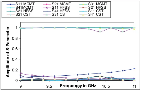
7. NUMERICAL RESULTS AND DISCUSSION

(7)

been compared with CST Microwave Studio simulated data and HFSS simulation data in Fig. 3.

0 0.2 0.4 0.6 0.8 1

9 9.5 Frequency in GHz10 10.5 11

A

m

p

litu

d

e

o

f

S

-P

ar

a

m

et

er

S11 MCMT S21 MCMT S31 MCMT S41MCMT S11 HFSS S21 HFSS S31 HFSS S41 HFSS S11 CST S21 CST S31 CST S41 CST

Figure 3. Comparison of theoretical, CST Microwave Studio And HFSS simulated data for an H-plane WR-90 waveguide two channel joints with a gap of 0.3 mm.

MATLAB codes have been written for analyzing the structure and numerical data have been obtained after running the codes. The structure was also simulated using CST microwave studio and HFSS. The theory has been validated by the excellent agreement between the theoretical, CST Microwave Studio simulated data and HFSS data. The scattering parameters for the circuit, when excited through port-2, port-3 and port-4 have not been presented in this section because these are also provide same pattern of data as for port-1.

ACKNOWLEDGMENT

The support provided by Kalpana Chawla Space Technology Cell, IIT Kharagpur is gratefully acknowledged.

REFERENCES

1. Das, S. and A. Chakraborty, “A novel modeling technique to solve a class of rectangular waveguide based circuits and radiators,”

(8)

2. Panda, D. K. and A. Chakraborty, “Multiple cavity modeling of a feed network for two dimensional phased array application,”

Progress In Electromagnetics Research Letters, Vol. 2, 135–140, 2008.

3. Panda, D. K. and A. Chakraborty, “Analysis of a 2:1rectangular waveguide power combiner using multiple cavity modeling technique,”NCCT-08, Proceedings, 87–90, India, 2008.

4. Harrington, R. F., Time-Harmonic Electromagnetic Fields, McGraw-Hill Book Company, New York, 1961.

5. Collins, R. E., Field Theory of Guided Waves, IEEE Press, 1991. 6. Harrington, R. F.,Field Computation by Moment Methods, Roger

E. Krieger Publishing Company, USA, 1982.