GIS-Based Local Ordered Weighted Averaging: A Case Study in London, Ontario

(1)

Scholarship@Western

Electronic Thesis and Dissertation Repository

4-22-2013 12:00 AM

GIS-Based Local Ordered Weighted Averaging: A Case Study in

London, Ontario

Xinyang Liu

The University of Western Ontario

Supervisor

Dr. Jacek Malczewski

The University of Western Ontario Graduate Program in Geography

A thesis submitted in partial fulfillment of the requirements for the degree in Master of Science © Xinyang Liu 2013

Follow this and additional works at: https://ir.lib.uwo.ca/etd

Part of the Geographic Information Sciences Commons

Recommended Citation Recommended Citation

Liu, Xinyang, "GIS-Based Local Ordered Weighted Averaging: A Case Study in London, Ontario" (2013). Electronic Thesis and Dissertation Repository. 1227.

https://ir.lib.uwo.ca/etd/1227

This Dissertation/Thesis is brought to you for free and open access by Scholarship@Western. It has been accepted for inclusion in Electronic Thesis and Dissertation Repository by an authorized administrator of

(2)

(Thesis format: Monograph)

by

Xinyang Liu

Graduate Program in Geography

A thesis submitted in partial fulfillment of the requirements for the degree of

Master of Science

The School of Graduate and Postdoctoral Studies The University of Western Ontario

London, Ontario, Canada

(3)

ii

Abstract

GIS-based multicriteria analysis is a procedure for combining a set of criterion maps and

associated criterion weights to obtain an overall value for each spatial unit (location) in the

study area. Ordered Weighted Averaging (OWA) is a generic algorithm of multicriteria

analysis. It has been integrated into GIS and applied for tackling a wide range of spatial

problems. However, the conventional OWA method is based on an assumption of spatial

homogeneity of its parameters. Therefore, it is referred to as a global model. This thesis

proposes a local form of OWA. The local model is based on the range sensitivity principle. A

case study of examining spatial patterns of socioeconomic status in London, Ontario is

presented. The results show that there are substantial differences between the spatial

patterns generated by the global and local OWA methods.

Keywords

Multicriteria analysis, local ordered weighted averaging (OWA), geographic information

(4)

iii

Acknowledgments

First of all, I want to express my gratitude to my supervisor Professor Jacek

Malczewski. Without his vivid explanations, his fruitful discussions, expertise and

enthusiasm in supervision, this thesis would not have been possible. He is the one who

guided me through the mist so that I can gain so much insight into my program and discover

the beauty of science. All the support he gave me and all the encouragement kept me

marching on. I especially admire his high efficiency and direct style that deeply inspire me

and make my early graduation possible. I’m truly grateful for everything that he teaches me,

which is going to be beneficial for a whole lifetime. In these years, I have always enjoyed

working with Professor Malczewski and feel honored to be one of his students.

I also want to dedicate this work to my family. Every parent loves their child, but not all of

them have to suffer the pain of being apart from each other. I have not been home for

nearly two years, and I can sense how hard it is for my parents to go through this time,

although they hid it so well on every single call. They have never stopped loving me and

supporting me. Without their love, I would not have had the courage to face all the

difficulties and finish this work. Please let me dedicate this work as well as my deepest love

to them.

Sirius Zhong is another person to whom I always desire to express my gratitude. His

friendship, his company, his unconditional help and his encouragement in both research

and life will be imprinted in my heart. From day one when I arrive in Canada, he has been

taking care of me. He manages to make it much easier for me to part with my family and

find some comfort in here. I am extremely lucky to have met him and had those many

beautiful memories with him.

Mohammadreza Jelokhani Niaraki, Qin Xue and Rui Hu have offered me enormous help that

will never fade away in my heart. My research will have not gone so smoothly without their

assistance. The help from Daniel Bednar in proofreading my thesis is also greatly

(5)

iv

Santiago and Autumn Gambles; we share wonderful memories behind us and may we all

have glorious future before us.

To my defense committee members (Dr. Diana Mok, Dr. Lu Xiao and Dr. Micha Pazner), I am

very proud and honored to have you as my committee. My gratitude always goes to your

suggestions and recommendations.

Last but not least, I am grateful for all the professors, administrative staff and fellow

students in the geography department. It is all of you who make this department a warm

(6)

v

List of Tables

Table 2-1 Example of Evaluation Matrix ... 7

Table 3-1 Pairwise Comparison Matrix ... 13

Table 3-2 Scale for Pairwise Comparison (Source: Saaty, 1980) ... 14

Table 3-3 Illustrative Example: calculating ordered criterion ... 15

Table 3-4 Properties of Regular Increasing Monotone Quantifiers with selected values of Parameter ... 17

Table 4-1 Criteria for Evaluating Socioeconomic Status in London, Ontario... 31

Table 4-2 A Scenario for Global Criterion Weighting: Pairwise Comparison Matrix ... 32

Table 4-3 Global Criterion Weights ... 32

Table 4-4 Neighborhood Scheme ... 35

Table 4-5 Neighborhood Attribute Table Based on Boundary Method ... 36

Table 4-6 The ORness and trade-off of different OWA operators for global and local order weights ... 52

(10)

ix

List of Figures

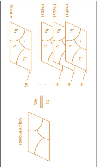
Figure 2-1 Example of Spatial MCA ... 8

Figure 3-1 Global OWA Procedure ... 11

Figure 3-2 Evaluation Strategy Space: the relationship between the measures of ORness and trade-off (Source: Eastman, 1997) ... 20

Figure 3-3 Local OWA Procedure ... 22

Figure 3-4 Identifying Neighborhood Using the Distance Based Method ... 24

Figure 3-5 Identifying Neighborhood Using the Boundary Based Method ... 24

Figure 4-1 The Study Area: London, Ontario (Source: Google Earth) ... 29

Figure 4-2 Global OWA: Standardized Criterion Maps ... 34

Figure 4-3 Local Standardized Criterion Maps Based on the Boundary ... 38

Figure 4-4 Local Standardized Criterion Maps Based on 850m Distance ... 39

Figure 4-7 The Comparison of Global and Local Standardized Criterion Maps for Average Dwelling Value Criterion ... 43

Figure 4-8 Local Weights Based on the Boundary ... 45

Figure 4-9 Local Weights Based on 850m Distance ... 46

Figure 4-10 Local Weights Based on 1600m Distance ... 47

(11)

x

Figure 4-12 The Comparison For Global and Local Criterion Weights of AVE_DWE ... 50

Figure 4-13 Output Maps of Global OWA Method ... 54

Figure 4-14 Output Maps of Local OWA based on Boundary Neighborhood Scheme ... 57

Figure 4-15 Output Maps of Local OWA based on 850m Neighborhood Scheme ... 58

Figure 4-16 Output Maps of Local OWA based on 1600m Neighborhood Scheme ... 59

Figure 4-17 Output Maps of Local OWA based 2400m Neighborhood Scheme ... 60

Figure 4-18 WLC Results of Global OWA Method and Local OWA Methods Based on Different Neighborhood Schemes ... 62

Figure 4-19 Spatial Autocorrelation Statistics ... 64

Figure 4-20 Scatter Plots of Global WLC and Local WLC ... 65

Figure 4-21 Selections from the Scatter Plot (Global WLC vs. Local WLC) ... 67

Figure 4-22 Selections from Scatter Plots (Global WLC vs. Local WLC) ... 68

(12)

xi

(13)

xii

(14)

xiii

(15)

Chapter 1

1

Introduction

Multicriteria Analysis (MCA) is a systematic procedure for evaluating a set of decision

alternatives based on multiple criteria. It has emerged as an area of research within the

field of environmental economics and regional planning in the early 1970s (Carver,

1991). Over the last two decades there has been substantial growth of MCA applications

(Wallenius et al., 2008). Decision or evaluation problems that involve geographical

(spatial) data are referred to as spatial decision problems. This type of problems is

typically tackled with the use of Geographic Information Systems (GIS). However, GIS

has limited capability for handling preferential information (such as preferences with

respect to relative importance of evaluation criteria). This limitation can be addressed

by integrating GIS and MCA (Malczewski, 1999; Chakhar and Mousseau, 2008).

A number of GIS-based MCA (GIS-MCA) methods have been developed over the last two

decades or so. These include weighted linear combination (WLC) (Eastman et al., 1993;

Malczewski, 2000; Mahini and Gholamalifard, 2006), ideal point methods (Carver, 1991;

Jankowski, 1995), analytical hierarchy process (Banai 1993; Rinner and Taranu, 2006)

and outranking analysis (Joerin et al., 2001; Chakhar and Mousseau, 2008). Among these

procedures, WLC and Boolean overlay approaches are considered as the most

straightforward and are most often employed (Malczewski, 1999). Boolean overlay

approaches apply the logical operators such as intersection (AND) and union (OR) on

Boolean maps to assess criteria (Jiang and Eastman, 2000). Yager (1988) generalized

these approaches and introduced a MCA method based on the ordered weighted

(16)

1.1 The Significance of GIS-based OWA

The main rationale for integrating GIS and OWA is that the two sets of methods have

unique and complementary capabilities for tackling spatial decision problems. On one

hand, GIS is efficient at storing and managing data, analyzing spatial information and

visualizing outcomes. On the other hand, OWA is a generic MCA procedure that

provides a platform for analyzing, evaluating, and prioritizing decision (or evaluation)

strategies (Malczewski, 1999; Rinner and Malczewski, 2002).

GIS-based OWA provides a tool for generating and visualizing a wide range of

multicriteria evaluation strategies by applying different operators and associated set of

ordered weights. The strength of OWA is that it can efficiently generate a set of diverse

solutions by changing the set of ordered weights. The OWA method not only provides a

single “optimal” solution, but can also generate a combination of solutions that can be

further examined for developing decision or evaluation scenarios.

1.2 The Limitation of Conventional OWA

In the last two decades, GIS-based OWA has been widely applied for solving a variety of

spatial problems including: use-land suitability problems (Eastman 1997; Malczewski,

2006b; Chen, et al., 2009 ), site-selection problems (Rinner and Raubal, 2004; Valente,

2008; Ekmekçioĝlu, et al., 2010), heat vulnerability assessment (Rinner, et al., 2010),

urban water management (Makropoulos et al., 2003), natural hazards (Gorsevski, et al.,

2010), and personal route planning (Nadi and Delavar, 2011). However, the limitation of

previous researches should be noted. The conventional OWA approach applied in

previous studies is regarded as “global OWA” because of the underlying assumption

about spatial homogeneity of the OWA parameters. The procedures of GIS-MCA,

including GIS-OWA, have mostly been derived from the general theory of decision

analysis (Malczewski, 1999) rather than from spatial theories. Consequently, the

(17)

method is based on an assumption that there is spatial homogeneity within the study

area. For instance, in the conventional GIS-OWA procedure, every alternative (location)

is assigned the same criterion weight. The conventional procedure uses a single value

function for the whole study area ignoring the fact that the form of the function may

depend on the local context (Malczewski, 2011). Therefore, all the previous studies are

based on the global OWA method and do not involve an explicit spatial representation

of local contexts.

Both Feick and Hall (2004) and Malczewski (2011) have addressed this limitation of

global GIS-MCA. Feick and Hall (2004) adopt an easy-to-use procedure to examine

weight sensitivity in both criteria and geographic space. They demonstrate a method for

visualizing the spatial dimension of criteria weight sensitivity by mapping the weight

sensitivity in order to detect localized variations of outcomes. Malczewski (2011)

introduces the concept of local weighted linear combination (WLC) to advance the

global WLC method, using the range sensitive principle as a core concept for developing

the local form of WLC model. However, there has been no attempt to develop the local

OWA method. This research is designed to fill this gap in the GIS-OWA studies.

In sum, OWA method is a generic GIS-MCA procedure. The conventional OWA method is

based on an assumption of spatial homogeneity. Consequentially, the conventional

OWA is referred to as the global OWA method. This research aims at advancing the

global OWA approach by developing a new OWA method to take into account the

spatial homogeneity. This new method is called local OWA.

1.3 Research Objectives

(18)

(1) To develop a local form of the OWA method. This objective will be achieved by

developing a new algorithm for transforming the global OWA to local OWA using the

range sensitivity principle.

(2) To examine the results of the local and global OWA using a case study of

(19)

Chapter 2

2

Theoretic Background

This chapter provides a theoretical background of GIS-MCA methods. It includes the

concept of MCA and spatial MCA.

2.1 Multicriteria Analysis

Multicriteria analysis (MCA) is a set of methods and procedures for evaluating decision

alternatives on the basis of multiple, conflicting criteria and selecting the best

alternative(s) (Voogd, 1983; Janssen and Rietveld, 1990). Criterion is a generic term that

includes both the concept of attributes and objectives (Malczewski, 1999). Hence

multicriteria analysis can be classified into two types: multiobjective and multiattribute

analysis.

Objective is a statement about the desired state of the system under consideration (e.g.,

land-use pattern, spatial pattern of transport facilities, location of public services, spatial

pattern of socioeconomic status, etc.). Objectives are functionally related to, or derived

from a set of attributes, indicating the direction towards which the attributes should be

optimized. Each objective represents one aspect of the desired state of the system. A

set of objectives should summarize all relevant concerns for achieving an overall goal of

the decision or evaluation problem. The multiobjective analysis is a model-oriented,

where the alternatives must be designed using the methods of mathematical

programming (Janssen and Rietveld, 1990; Malczewski, 1999).

Attribute is a measurable characteristic of an object (decision alternative, location, area,

etc.). It is a descriptive value (Drobne and Lisec, 2009). It aims at assessing the degree to

which a given objective might be achieved (Pitz and McKillip, 1984). Attributes are used

(20)

means or information sources available to the decision maker for formulating and

achieving the decision maker’s (or expert’s) objectives (Starr and Zeleny, 1977).

Multiattribute analysis is based on the assumption that the set of alternatives are

known. The core of solving multiattribute decision problems is the evolution of (and

choice among) alternatives described by their attributes. For the most part, GIS-MCA

belongs to the multiattribute analysis (Malczewski, 2006). This research is concerned

with multiattribute analysis. Hereafter, the terms multiattribute analysis and

multicriteria analysis will be used interchangeably.

2.2 Spatial Multicriteria Analysis

Spatial MCA focuses on geographically defined decision alternatives which are evaluated

by a set of criteria (Carver, 1991; Jankowski, 1995; Malczewski, 1999). The kernel of

spatial MCA is the integration of MCA and GIS methods. Conventional MCA can be used

to deal with the complexity of the real world problems that may involve a large number

of alternatives and multiple and conflicting evaluation criteria. Nevertheless, to solve

spatial decision problems, MCA also requires spatial analytical functions and the

capacity of processing geographic data. This calls for the integration MCA and GIS.

In spatial multicriteria analysis or GIS-MCA, attributes, represented as map layers, are

the properties of geographical entities; hence attributes can be interpreted as criteria

(criterion maps). The weight associated with a criterion map represents the preference

of decision makers (or experts). It indicates the relative importance of criteria. The

spatial units (locations or areas) represent the decision (or evaluation) alternatives. In

the raster data, each raster cell or a combination of cells is considered as an alternative.

In the vector data, alternatives are represented by points, lines, polygons or a

combination of these three spatial objects.

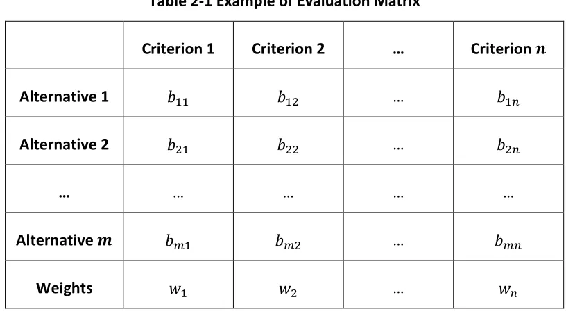
An evaluation matrix can be formed to represent the relationships between alternatives

(21)

= 1,2,…, ; where and are the number of alternatives and criteria, respectively. The

criterion weights ( ) are shown in the last row. In the spatial MCA, the evaluation

criteria are associated with geographical entities therefore can be represented in the

forms of maps (see Figure 2-1).

Table 2-1 Example of Evaluation Matrix

Criterion 1 Criterion 2 … Criterion

Alternative 1 …

Alternative 2 …

… … … … …

Alternative …

Weights …

A criterion map consists of a set of polygons. Each polygon stands for an alternative in

the evaluation matrix and is described by a set of criterion values (that is, the -th

alternative or polygon is described by for k = 1,2,…, ). Criterion weights are assigned

to each criterion maps. Given the set of criterion maps and associated criterion weights,

the input data can be processed by GIS techniques and MCA methods to obtain the

(22)

(23)

2.3 GIS-based OWA Method

GIS-based OWA method is the combination of GIS techniques and OWA method.

Eastman (1997) first extended the concept of OWA to GIS application to establish the

decision support model in Idrisi-GIS. In the recent decade, many researches focus on

integrating OWA concept and GIS application to practical problems (Jiang and Eastman,

2000; Malczewski, 2000; Rasmussen et al., 2002; Araújo and Macedo, 2002; Chen et al.,

2009; Charabi and Gastili, 2011; Feizizadeh and Blaschke, 2012).

Criterion values, criterion weights and order weights are three important elements of

OWA. Criterion values are the presentation of attributes. The criterion weights indicate

the importance of each criterion. The order weights are assigned to each reordered

criterion after the reordering process. The determination of order weights is critical on

integrating GIS and OWA (Malczewski, 2006c). Jiang and Eastman (2000) demonstrated

the Idrisi-OWA procedure but failed to provide a method for obtaining the order

weights. Consequently, several researches proposed methods for generating the

optimal order weights: based on the degree of ORness and trade-off (Asproth et al.,

1999; Mendes and Motizuki, 2001; Rasmussen et al., 2002), based on the principles of

maximum dispersion or the maximum trade-off (Rinner and Malczewski, 2002;

Malczewski et al., 2003; Malczewski, 2006c). The approach of maximum trade-off can be

implemented by parameterized OWA. This research applied a linguistic quantifier by

using the parameter to determine the order weights (see Section 3.1.5). The

generality of OWA is related to its capability to implement different OWA operators by

(24)

Chapter 3

3

Methods

This chapter consists of two sections: the implementation of global OWA method and

the development of local OWA approach.

3.1 Global OWA Method

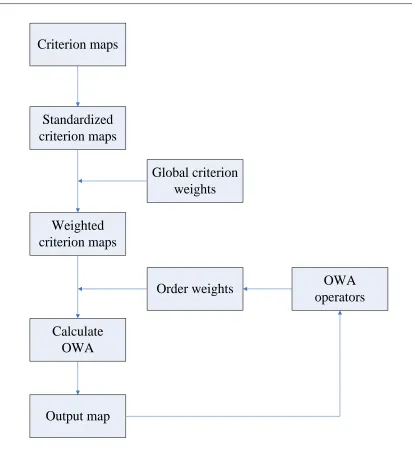
3.1.1 Global OWA Procedure

The global or conventional OWA method applies a weighted sum of ordered evaluation

criteria including a set of alternatives (or locations) and a set of evaluation criteria. Each

alternative, , is described by a set of standardized criterion (or attribute) values ( ),

for = 1, 2, … , , and = 1, 2, … , . The OWA is composed of two types of weights:

criterion weights ( ) and ordered weights ( ). The global criterion weights: ( , ∑ = 1) are applied to specific criteria. They represent

the preferences (of the decision maker or expert), with respect to each criterion to

indicate its relative importance. On the other hand, order weights,

( ; ∑ ), are assigned to ordered criteria associated with criterion

(25)

Criterion maps

Standardized

criterion maps

Weighted

criterion maps

Global criterion

weights

Order weights

Calculate

OWA

operators

Output map

(26)

The procedure of global OWA involves the following steps (see Figure 3-1):

(1) standardize criterion values of each criterion maps;

(2) define the global criterion weights according to the preferences of experts;

(3) sort weighted standardized criterion values of each location in descending order;

(4) order global criterion weights according to the ordered criterion values for each

location;

(5) select appropriate ordered weights by adopting different OWA operators;

(6) multiply the weighted standardized values by corresponding order weights;

(7) sum up the products to obtain an overall OWA score for each location.

3.1.2 Standardizing Criterion Maps

The first step of any MCA is to collect relevant data and information about the decision

or evaluation problem. In GIS-MCA, the input data is typically represented in the form of

criterion maps. Since the various criteria are likely to be measured in different system,

the criterion maps must be transformed into a standardized scale (Carver, 1991). The

method for transforming criterion maps into standardized forms is defined as follows:

(3-1)

for -th criterion to be minimized; (3-2)

for -th criterion to be maximized (3-3)

where, refers to the raw (unstandardized) criterion value; and

indicate the maximum and minimum criterion value of the -th criterion, respectively;

is the global range of the -th criterion; is the standardized criterion value,

ranging from 0 to 1, where 0 is the least-desired value, while 1 indicates the

(27)

perform the criterion standardization (e.g., a benefit criterion). Equation 3-3 should be

applied for criterion to be minimized (e.g., a cost criterion).

3.1.3 Deriving Criterion Weights using Pairwise Comparisons

Some criteria are more important than the others. The criterion weights estimate the

perceived importance of individual criterion relative to the other criteria (Carver, 1991).

The pairwise comparison method is applied to estimate criterion weights (see Table 3-1).

Table 3-1 Pairwise Comparison Matrix

Criterion 1 Criterion 2 … Criterion n

Criterion 1 1 p12 … p1n

Criterion 2 p21 = 1/p12 1 … p2n

… … … … …

Criterion n pn1 = 1/p1n pn2=1/p2n … 1

In the pairwise comparison method, the pairwise comparison matrix should be

developed first (Table 3-1). Comparing each pair of criteria, decision maker (or expert)

evaluates the relative importance of criteria using the scale shown in Table 3-2. For

instance, if criterion 1 is moderately more important than criterion 2, then p12 = 4; the

comparison value of p21 is calculated using the reciprocal principle (that is, p 21 = 1/p12 =

0.25). Note that the cells on the diagonal in the pairwise comparison matrix have the

same values of 1 because pairwise comparisons represented of those cells are between

a given criterion and itself. Given the pairwise comparison matrix, the pairwise

(28)

then the criterion weight is calculated as an average value of the normalized pairwise

comparisons (see Section 4.3.2).

Table 3-2 Scale for Pairwise Comparison (Source: Saaty, 1980)

Intensity of

Importance Definition

1 Equal importance

2 Equal to moderate importance

3 Moderate importance

4 Moderate to strong importance

5 Strong importance

6 Strong to very strong importance

7 Very strong importance

8 Very to extremely strong importance

9 Extreme importance

3.1.4 Sorting Weighted Criteria

The next step is to generate ordered criteria ( ). This is achieved by sorting the

weighted standardized criterion values ( ) for each alternative or location in a

descending order (Yager, 1988; Malczewski and Rinner, 2005). Table 3-3 illustrates the

procedure using a set of four alternatives (locations), three standardized criterion

( ), and associated criterion weights ( = 0.2, =0.5, = 0.3).

The standardized criteria are weighted by multiplying the associated criterion weights.

Further, the weighted criterion values ( ) are sorted in a descending order. The

(29)

of weighted criterion values ( = 0.0, = 0.45, = 0.18) associated with

= 1 is arranged in the descending order as follows: = 0.45, = 0.18, = 0.0.

Since the criterion values are shuffled, the corresponding criterion weights are also

rearranged in the sorting process. These rearranged criterion weights form a new matrix,

the ordered criterion weight ( ). The ordered criterion weights are used to

determinate the ordered weights (see Section 3.1.5). The procedures of sorting criterion

values and generating ordered criterion weights have been implemented in a Local MCA

Calculator (see Appendix).

Table 3-3 Illustrative Example: calculating ordered criterion ( )

Criteria

{0.0, 0.7, 1.0 ,0.4} 0.2 {0.0, 0.14, 0.2, 0.08}

{0.9, 0.3, 0.2, 0.6} 0.5 {0.45, 0.13, 0.01, 0.3}

{0.6, 0.8, 0.1, 0.3} 0.3 {0.18, 0.24, 0.03, 0.09}

Criteria

{0.5, 0.3, 0.2, 0.5}

{0.3, 0.2, 0.3, 0.3}

{0.2, 0.5, 0.5, 0.2}

{0.45, 0.24, 0.2, 0.3}

{0.18, 0.14, 0.03, 0.09}

(30)

3.1.5 Determining Order Weights

3.1.5.1 Fuzzy linguistic quantifiers

The order weights can be estimated using a number of methods (Yager, 1996). The

linguistic quantifier-based method is one of the most often used in OWA applications.

Linguistic quantifiers can be represented as a fuzzy set (Zadeh, 1983). Consequently, the

term linguistic and fuzzy quantifiers can be used interchangeable. Translating natural

language specifications into mathematics formulas is the core purpose of fuzzy

quantifiers. Yager (1996) proposed a procedure for quantifier-guided MCA that fuzzy

linguistic quantifiers were used to specify the statement about the number (proportion)

of criteria to be satisfied by applying OWA operators (e.g., all criteria must be satisfied,

most of the criteria should be satisfied or at least half of criteria should be satisfied).

To determine the values of order weights, the associated quantifier Q needs to be

specified first. There are two generic classes of linguistic quantiﬁers: absolute and

relative quantiﬁers (Zadeh 1983; Yager 1996). The statements such as “about ﬁve” or

“more than ten” belong to the class of absolute quantifiers; they are deﬁned as fuzzy

subsets of [0, ]. The relative quantifiers are closely related to imprecise proportions.

They are deﬁned as fuzzy subset of [0, 1] with proportional terms such as “a few”, “half”,

“many”, “most”. Therefore, the relative quantifier can be identified by one of the

simplest and the most often used method to parameterize subset on the unit interval as

following (Yager, 1996):

( ) (3-4)

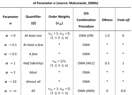
The ( ) represents a fuzzy set in interval [0, 1], including monotonically increasing

proportions of elements. Hence the whole family of regular increasing monotone (RIM)

quantifier can be generated from this quantifier ( ). Consequently, by changing the

value of parameter , one can obtain a wide range of aggregation operators. Specifically,

(31)

between the two extreme cases of the “at least one” and “all” quantifiers (see Table 3-4)

(Malczewski and Rinner, 2005). For instance, when the value of parameter tends to be

zero, the quantiﬁer ( ) approaches its extreme case of “at least one”. When the value

of parameter approaches infinity, the quantifier ( ) approaches its extreme case of

“all”. Using the parameter , the order weights can be defined as follows (Yager, 1996;

Malczewski, 2006b):

(∑ ) (∑ ) (3-5)

where is the order weight for the k-th criterion associated with the -th location;

is the ordered criterion weights; is the parameter associated with the fuzzy quantifier.

Table 3-4 Properties of Regular Increasing Monotone Quantifiers with selected values

of Parameter (source: Malczewski, 2006b)

Parameter Quantifier

(𝑸) Order Weights (𝒗 ) GIS Combination Procedure

ORness Trade-off

→ 0 At least one = 1; = 0,

( < ≤ ) OWA (OR) 1.0 0

→ 0.1 At least a few * OWA * *

→ 0.5 A few * OWA * *

→ 1 Half (identity) = 1/ ,

( ≤ ≤ ) OWA (WLC) 0.5 1

→ 2 Most * OWA * *

→ 10 Almost all * OWA * *

→ All = 1; = 0,

( ≤ < ) OWA (AND) 0 0.0

Note: * the set of order weights depends on values of sorted criterion weights and

(32)

3.1.5.2 OWA operators

The generality of OWA method is related to its ability of implementing a wide range of

combination operators by selecting an appropriate set of order weights (Yager 1988).

The combination operators are called OWA operators. They include the weighted linear

combination (WLC) and Boolean overlay operations such as intersection (AND) and

union (OR) (Yager 1988; Jiang and Eastman, 2000). The AND and OR operators are the

most often used GIS combination procedures.

In fact, the set of order weights determinates the type of the OWA operator. In the

practical application, the AND and OR operators represent the two extreme situations.

For example, when parameter ( → ), the order weights are generated as . This extreme case represents the Boolean OR

combination (see Table 3-4). If parameter = 0.001 ( → 0), only the lowest values are

selected by the OWA operator because the order weights ;

this is an equivalent of the AND type of Boolean combination (see Table 3-4).

Moreover, the WLC operator is determined by a set of equal order weights

( ); that is, the identity quantifier or parameter = 1 is

applied. Hence, the WLC operator does not change in the re-order weighted criterion

value because equal ordered weights are assigned to each ordered weighted criterion.

The AND, OR and WLC operators are only three ‘special’ cases. One can generate a large

number of OWA operators by changing the value of parameter or the quantifiers

ranging from “all” to “at least”.

One can use the measurements ORness and trade-off to classify the OWA operators

with respect to their positions between the AND and OR operators (Yager, 1988;

Eastman, 1997; Jiang and Eastman, 2000):

(33)

- = √ ∑( ) , 0 ≤trade-off≤ 1 (3-7)

ORness measures the degree similarity of an OWA operator to the logical OR in terms of

its combination behavior (Malczewski et al., 2003). The trade-off is a measurement for

the substitutability (or compensation) of low values on one criterion by high values on

other criterion (Jiang and Eastman, 2000). It indicates the degree of how a good

performance on one criterion under consideration compensates a poor performance on

other criterion (Malczewski et al., 2003). The value of zero conveys no trade-off among

criteria and the value of one indicates a full trade-off.

3.1.5.3 Evaluation strategy space

Evaluation (or decision) strategy space can be formed by two measurements: ORness

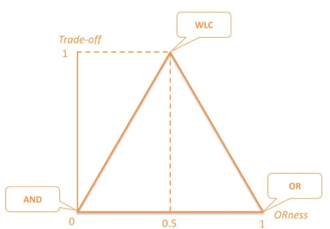
and trade-off (Jiang and Eastman, 2000; Rinner and Malczewski, 2002). Figure 3-2 shows

the relationship between ORness and trade-off. The shape of evaluation strategy space

depends on the number of criteria ( ). When two criteria are involved in the evaluating

process, the strategy space has a triangle shape (Figure 3-2). The three vertices of the

triangle represent the three extreme cases of the OWA operators: AND, OR and WLC

(see Figure 3-2). For instance, the top vertex represents the WLC operator ( = 1),

characterized by an intermediate degree of ORness and full trade-off.

As the number of criteria increases from = 2 to → , the shape of decision strategy

space changes to a rectangular form (Malczewski and Rinner, 2005). Specifically under a

given degree of ORness, more criterion maps are involved in the procedure and this

leads to the higher level of trade-off, except for the extreme cases of OWA operators

(AND, OR and WLC operators). For AND, OR and WLC operators, the measures of

trade-off and ORness are fixed irrespectively of the number of criterion maps (Malczewski and

(34)

Figure 3-2 Evaluation Strategy Space: the relationship between the measures of

ORness and trade-off (Source: Eastman, 1997)

3.1.6 Defining Global OWA

For a given set of criterion maps, the function of OWA scores is defined as follows (Yager,

1988):

∑ (3-8)

where is the overall OWA score of the -th location or alternative; is the

ordered weight; is the ordered weighted criterion value. The spatial pattern of OWA

scores can be displayed on a map. The location (alternative) with the highest overall

(35)

3.2 Local OWA Method

3.2.1 Local OWA Procedure

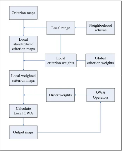
The local OWA procedure is illustrated in Figure 3-3. It starts with defining the set of

evaluation criterion maps. Next, a neighborhood scheme is specified. Based on the

neighborhood scheme, the range sensitivity principle is applied to obtain the local range

for each location in the study area. This is followed by performing the local

standardization for each criterion map. Then, the global criterion weights are estimated,

providing the basis for calculating local criterion weights. Particularly, the local criterion

weight associated with a given location is a function of the global weight and the local

range. Given the local standardized criteria and local criterion weights, one can generate

local weighted criterion maps. Further, a set of order weights is defined based on the

specified value of parameter . Finally, the local weighted criteria maps and order

weights are combined to obtain the local OWA scores (output map).

The concept of the neighborhood, local range and local criterion weight are critical for

conveying spatial heterogeneity and local context. Therefore, the rest of this chapter

will focus on this concept. The order weights of the local OWA method are obtained in

the same way as in the global OWA approach (see Section 3.1.5). Therefore, the process

of selecting appropriate order weights by specifying different values of parameter is

(36)

Criterion maps

Local

standardized

criterion maps

Local weighted

criterion maps

Global

criterion weights

Order weights

Calculate

Local OWA

OWA

Operators

Output maps

Local range

Neighborhood

scheme

Local

criterion weights

(37)

3.2.2 Defining Neighborhoods

One of the crucial differences between the local and global OWA methods is the

utilization of the neighborhood scheme for localizing OWA method. In this research, an

alternative is a polygon (or location). Two approaches are applied to identify

neighborhoods: the distance-based method and the boundary-based method.

3.2.2.1 Distance-based neighborhood scheme

In the distance-based method, neighborhoods are generated based on the threshold

distance ( ). The centroid of each polygon must be found in order to measure the

distance between polygons (locations). The threshold distance is assigned according to

specific situation. Once the threshold distance is determined, one can compare the

threshold distance with the distances between focal polygon and other polygons. If the

distance between the focal location and its nearby polygon is smaller than the threshold

distance, then the polygon is defined as a neighbor of the focal polygon. The

neighborhood of focal location consists of the focal location and its neighbors. For the

local OWA method, the value of threshold distance must be large enough to guarantee

that each polygon has at least one polygon as its neighbor. This rule ensures that

the denominator of Equations 3-10, 3-11 and 3-12 is greater than zero. Moreover, if the

threshold distance is large enough to cover the whole study area, then the

neighborhood of each location contains all other locations in the study area. In this case,

the local and global OWA methods generate the same results.

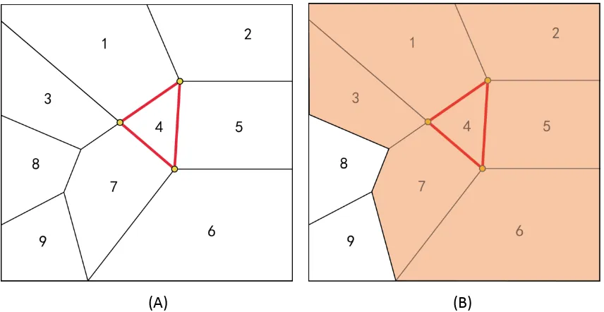
Figure 3-4 shows an example. The study area is represented in a vector format. Points

from 1 to 9 represent the centroids of nine polygons. In Figure 3-4-A, represents the

threshold distance and polygon 4 is the focal polygon. Since the straight line distances

between the centroid of polygon 4 and centroids of polygon 1, 5 and 7 are smaller than

the threshold distance ( ), polygons 1, 4, 5 and 7 form the neighborhood of the focal

(38)

(A) (B)

Figure 3-4 Identifying Neighborhood Using the Distance Based Method

3.2.2.2 Boundary-based neighborhood scheme

(A) (B)

Figure 3-5 Identifying Neighborhood Using the Boundary Based Method

In the boundary-based method, neighborhoods are defined as areas which share their

boundaries with the focal area. This research is based on the Queen’s case. If two

(39)

neighbors. Any polygon sharing boundaries with a given focal polygon is defined as the

neighbor of that area (see Figure 3-5). For example, the polygon 4 shares three points

and three lines with surrounding polygons (see Figure 3-5-A), therefore polygon 1 to 7

form the neighborhood of polygon 4 (see Figure 3-5-B).

3.2.3 Range Sensitivity Principle and Local Range

The range sensitivity principle is used as a core concept for developing the local form of

OWA method. The range sensitivity is a normative property with respect to the

dependence of criterion weights on the ranges of criterion values (von Nitzsch and

Weber 1993; Fischer, 1995; Malczewski, 2011). In the global OWA method, an

assumption about uniformity of preferences over the whole study area is applied to

global criterion weights. In the process of global standardization, the global

standardized criterion value ( ) is the function of global range ( ) (see Equation 3-2

and 3-3). The global range is the parameter that is defined for the whole study area. It

implies that the spatial heterogeneity is ignored, irrespectively of the local context and

factors that may affect the level of worth associated with a particular criterion value.

The range sensitivity principle assumes that for a given criterion the greater the range of

the criterion values is, the greater the weight of importance assigned to the criterion

should be (von Nitzsch and Weber 1993; Fischer, 1995). To convey local context in the

specific neighborhood, the local range can be generated based on this principle. The

local range ( 𝑞) is defined as the difference between the maximum and minimum

criterion values in the 𝑞q-th neighborhood for the -th criterion. Formally:

𝑞

𝑞{ 𝑞} 𝑞{ 𝑞} (3-9)

where 𝑞{ 𝑞} and 𝑞{ 𝑞} are the minimum and maximum values of the -th

criterion in the q-th neighborhood; 𝑞 is the local range of the -th criterion in the q-th

(40)

3.2.4 Local Standardization

The values of each criterion are standardized locally as follows:

𝑞

for the -th criterion to be minimize; (3-10)

𝑞

for the -th criterion to be maximize (3-11)

where 𝑞{ 𝑞} and 𝑞{ 𝑞} are the minimum and maximum values of the 𝑞-th

neighborhood for the k-th criterion; 𝑞 is the local range; 𝑞 is the locally standardized

criterion values, ranging from 0 to 1, where 0 is assigned as the least-desired criterion

value and 1 is assigned as the most-desired value in the q-th neighborhood.

3.2.5 Local Criterion Weights

The value of local criterion weight depends on the scheme used for subdividing a study

area into neighborhoods (zones or regions). Local criterion weight ( 𝑞) can be obtained

as follows:

𝑞

∑

≤ 𝑞 ≤ and ∑ 𝑞 (3-12)

where 𝑞 is the local criterion weight associated with the q-th neighborhood for the

-th criterion; is the global criterion weight of -th criterion; is the global range,

which equals to the maximum minus the minimum criterion value in the -th criterion; 𝑞

is the local range. Since the value of local weight depends on the neighborhood

scheme, it is also referred to the neighborhood-based criterion weights (Feick and Hall

(41)

3.2.6 Sorting Local Weighted Criteria

Unlike global criterion weights ( ), which are presented as an array, the local weights

( 𝑞) form a matrix. It implies that each location (spatial unit) on the criterion map has

assigned a corresponding value of the local weight. The calculation process of weighting

local criterion maps involves the matrix multiplication of standardized criterion values

and local criterion weights. The procedure for sorting (ordering) local weighted criteria

is the same as the sorting method for the global OWA method (see Section 3.1.4). Thus,

one can sort the weighted criterion values ( 𝑞 𝑞) to obtain the ordered weighted

criterion values ( 𝑞)

3.2.7 Generating Local Order Weights

In the local OWA method, the procedure of generating local order weights is the same

as of determining order weights in the global OWA method (see Section 3.1.5).

According to Equation 3-5, the order weights ( ) are derived from ordered criterion

weights ( ). Although the local criterion weights ( 𝑞) are different from global

criterion weights ( ), both weights are formed as a matrix. In the local OWA method,

the order weights are defined as follows:

𝑞 _(∑ 𝑞

) (∑ 𝑞) (3-13)

where 𝑞 is the local order weight; 𝑞 is the ordered weighted local criterion values for

the -th criterion in the 𝑞-th neighborhood; is the parameter associated with the fuzzy

(42)

3.2.8 Calculating Local OWA

The calculation of local OWA scores is defined as follows:

𝑞 _∑ 𝑞

𝑞 (3-14)

where 𝑞 is the overall local OWA score for the 𝑞-th neighborhood; 𝑞 is the local

order weights (see Section 3.2.7); 𝑞 is the ordered weighted local criterion values for

the -th criterion in the 𝑞-th neighborhood(see Section 3.2.7).

3.3 Comparing Local OWA methods and Global OWA methods

The most important difference between local and global OWA methods lies in applying

different criterion weights. In the global OWA method, the relative importance of

evaluation criterion is the only factor to determine the criterion weights, defined as the

global weights. In the local OWA method, however, the local criterion weights are

estimated on the basis of the preferences with respect to relative importance of criteria

and the local context. In addition, the local weights can be considered as the adjusted

global weights depending on the definition of neighborhoods. To be more specific, the

local criterion weight is the function of the global criterion weight modified by the

relationships between the local and global ranges. The ranges in turn depend on the

(43)

Chapter 4

4

Case Study

The aim of the case study is to test the local OWA method and to compare the results of

global and local OWA methods by evaluating the socioeconomic status of

neighborhoods in London, Ontario.

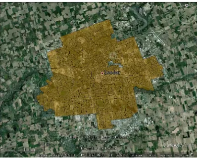
4.1 The Study Area

The study area is the City of London, Ontario (see Figure 4.1). London is located in

Southwestern Ontario. It is situated along the Quebec City - Windsor corridor. The city

of London has a population of 366,151 (Statistics Canada, 2011).

(44)

4.2 Data Sources

The geographic data of the study area is obtained from a secure website database

distributed through the university’s library system (UWO, 2011). The geographic data

are in the vector format; that is, the census dissemination area is represented by

polygons. ArcMap 10.0 is applied to manipulate the spatial data.

The socioeconomic data for London was derived from the Population Census of 2006

(Statistics Canada, 2006). The census dissemination area is the basic unit of the analysis.

The statistic data for the evaluation criteria is available for 494 dissemination areas in

London, Ontario. The unpopulated Census Tract 0056 is excluded from the analysis.

4.3 The Application of OWA methods

4.3.1 Criteria Selection

The problem of evaluating socioeconomic conditions of residential neighborhoods (and

related problem of measuring quality of life or residential quality) provides a good

example of a situation in which one has to combine a number of evaluation criteria

(indicators) to obtain a composite measure of socioeconomic status. Many studies rely

on multivariate statistics and/or multicriteria evaluation procedures (Can, 1992; Raphael

et al., 1996; CUISR, 2000). The weighted linear combination (WLC) is the most often

used approach for obtaining a composite measure of quality of life (e.g. Raphael et al.,

1996; CUISR, 2000; Massam, 2002). The Federation of Canadian Municipalities (FCM)

provides a reporting system to monitor the quality of life in Canadian municipalities

(FCM, 1999; FCM, 2001). The project is known as the quality of life reporting system

(QOLRS). The selection of evaluation criteria for this case study of assessing the

socioeconomic status in London is based on the QOLRS. The set of criteria includes:

median incomes, incidence of low incomes, employment rate, average values per

(45)

criterion, the maximum type indicates that the higher value is more desired. The

minimum type means that the lower value of the criterion is more desired.

Table 4-1 Criteria for Evaluating Socioeconomic Status in London, Ontario

Name Description Type

1 MED_INC* Median incomes ($) Maximum

2 LOW_INC* Incidence of low income (%) Minimum

3 EMP_RAT* Employment rate (%) Maximum

4 AVE_DWE* Average value of dwelling ($) Maximum

5 UNI_EDU* University education

(% population 15 years and over) Maximum

6 RES_BUR** Residential burglary (relative risk ratio) Minimum

( Sources of data: * Statistics Canada, 2006 and ** Poetz, 2003)

4.3.2 Identify Global Criterion Weights

The global criterion weights represent the relative importance of criteria. To define the

global criterion weights, several scenarios are developed by applying the pairwise

comparison approach (see Section 3.1.3). For the purpose of demonstrating the OWA

procedures, this case study focuses on one of the criterion weighting scenarios. Table

4-2 shows the pairwise comparison matrix. The meaning of scores in the pairwise

comparison matrix is given in Table 3-2. The pairwise comparisons are normalized; that

is, each cell of the matrix is divided by its column total (the results are shown in Table

4-3). Then the global criterion weights are obtained by computing the average value of the

(46)

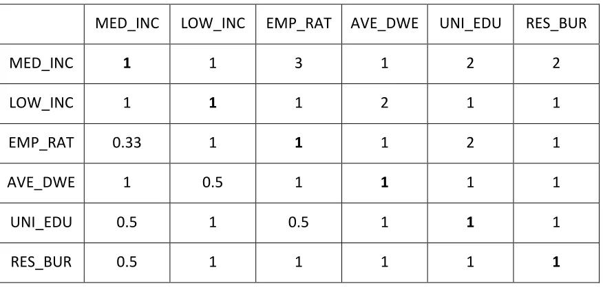
Table 4-2 A Scenario for Global Criterion Weighting: Pairwise Comparison Matrix

MED_INC LOW_INC EMP_RAT AVE_DWE UNI_EDU RES_BUR

MED_INC 1 1 3 1 2 2

LOW_INC 1 1 1 2 1 1

EMP_RAT 0.33 1 1 1 2 1

AVE_DWE 1 0.5 1 1 1 1

UNI_EDU 0.5 1 0.5 1 1 1

RES_BUR 0.5 1 1 1 1 1

Table 4-3 Global Criterion Weights

MED_INC LOW_INC EMP_RAT AVE_DWE UNI_EDU RES_BUR Weights

MED_INC 0.23 0.18 0.40 0.14 0.25 0.29 0.25

LOW_INC 0.23 0.18 0.13 0.29 0.13 0.14 0.18

EMP_RAT 0.08 0.18 0.13 0.14 0.25 0.14 0.15

AVE_DWE 0.23 0.09 0.13 0.14 0.13 0.14 0.14

UNI_EDU 0.12 0.18 0.07 0.14 0.13 0.14 0.13

RES_BUR 0.12 0.18 0.13 0.14 0.13 0.14 0.14

Sum 1.00 1.00 1.00 1.00 1.00 1.00 1.00

Note: theconsistency ratio CR = 0.06 < 0.1 indicates that the global criterion weights are

based on a consistent set of pairwise comparisons (see Section 3.1.3).

(47)

4.3.3 Global Standardization

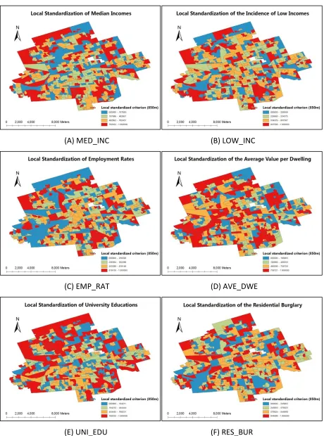
The six standardized global criterion maps are generated according to Equations 3-1, 3-2,

and 3-3 (see Figure 4-2). The Jenks natural breaks classification method is applied to

display criterion maps, where classes are developed on natural groupings inherent in

the data. The class breaks are statistically determined by best grouping similar values

and maximizing the differences between classes in ArcGIS 10.0 (ESRI, 2010). Boundaries

of divided classes are set according to the relatively ‘big jumps’ within data values. The

Jenks natural breaks classification method is applied to all criterion maps in this study.

In the outcome of global standardization, the criterion map of median incomes shows

that the northwestern of London has high values, while the central and southeastern of

the city are characterized by low values of median incomes (see Figure 4-2-A). A similar

spatial pattern can also be observed for criteria of average value per dwelling, university

education and residential burglary (see Figures 4-2-D, 4-2-E and 4-2-F). One can

conclude that the residential neighbourhoods in the northwest part of London are

characterized by higher median incomes, higher average value of dwelling, higher level

of education and lower residential burglary rates. Conversely, the central and southeast

sectors of the city tend to have lower median incomes, lower average value of dwelling,

lower level of education and higher residential burglary rates. For criterion maps of the

incidence of low income and the employment rate (see Figures 4-2-B and 4-2-C), the

spatial pattern is dispersed with a slight tendency of clustering higher values at the

(48)

(A) MED_INC (B) LOW_INC

(C) EMP_RAT (D) AVE_DWE

(E) UNI_EDU (F) RES_BUR

(49)

4.3.4 Neighborhood Scheme

This research applies two methods of the neighborhood scheme: distance-based and

boundary-based methods (see Section 3.2.2). ArcGIS 10.0 is used as the tool to establish

the neighborhood scheme (ESRI, 2010). Table 4-5 lists the four specific neighborhood

schemes applied in this case study.

Table 4-4 Neighborhood Scheme

Method Descriptions

Based on the distance

d = 850 m

d = 1600 m

d = 2400 m

Based on the boundary Queen’s case

(Note: d = threshold distance)

Implementing the distance-based method in ArcGIS involves two steps: (1) the “Feature

to Point” tool generates centroid points of polygons, and (2) the tool “Point Distance” is

applied to find neighbors according to the threshold distance. The output is a table that

contains the list of the focal polygons and information of about all near polygons

(centroids) within the search radius or threshold distance. Three threshold distances are

used: 850m, 1600m and 2400m (see Table 4-5). The threshold should be large enough

to guarantee that each location (polygon) has at least one neighbor. The distance of

850m is the smallest threshold to meet this constrain, and the distance of 2400m is

selected based on previous research (Malczewski and Poetz, 2005). The research

findings suggest that the processes underlying the relationships between some

socioeconomic variables in London, Ontario operate at a local (neighborhood) scale.

(50)

regression that the spatial variability in the relationships is significant at the spatial scale

associated with kernel bandwidths less than 2400 m.

The boundary-based method is another way to identify the neighborhood scheme (see

Section 3.2.2.2). Using the tool “Spatial Join” in ArcGIS 10.0 creates the neighborhood

attribute table for identifying neighborhoods based on shared boundaries (ESRI, 2010).

For instance, the neighborhood attribute table of the example showed in Figure 3-5 is

given in Table 4-5. The Neighbor column of the table indicates the number of polygons

which share the boundary with the target polygon.

Table 4-5 Neighborhood Attribute Table Based on Boundary Method

No. Target Neighbor No. Target Neighbor No. Target Neighbor

1 1 2 14 4 2 27 7 1

2 1 3 15 4 3 28 7 3

3 1 4 16 4 5 29 7 4

4 1 5 17 4 6 30 7 5

5 1 7 18 4 7 31 7 6

6 2 1 19 5 1 32 7 8

7 2 4 20 5 2 33 7 9

8 2 5 21 5 4 34 8 3

9 3 1 22 5 6 35 8 7

10 3 4 23 5 7 36 8 9

11 3 7 24 6 4 37 9 7

12 3 8 25 6 5 38 9 8

(51)

Based on the table of neighborhoods, generated by both the distance-base method and

the boundary-based method, one can compute the local range for each dissemination

area (polygon) according to Equation 3-9 (see Section 3.2.3). Since the calculation of the

local range cannot be accomplished in the ArcGIS, a calculator for computing the local

ranges is developed (see Appendix).

4.3.5 Local Standardization

Since four neighborhood schemes are applied in this case study, four sets of local

standardized criterion maps are generated by using Equations 3-10 and 3-11. Figure 4-3

shows the results of local standardization for six criteria according to the

boundary-based neighborhood scheme. The local standardized criterion maps boundary-based on

distance-based neighborhood scheme with the threshold distance of 850m, 1600m and 2400m

are showed in Figures 4-4, 4-5, and 4-6, respectively.

There are essential differences between the global standardized criterion map (Figure

4-2) and corresponding local criterion maps (Figures 4-3, 4-4, 4-5 and 4-6). As expected,

spatial patterns of criterion values generated by the local OWA method are more

localized than the global one. The AVE_DWE criterion (the average value per dwelling) is

used to illustrate the differences between the global and local patterns (see Figure 4-7).

This criterion has the distinct spatial pattern of the global standardization values (see

Section 4.3.3). The spatial pattern with the higher values in the northwestern part of

London can be observed for the global standardization (see Figure 4-7-A). However, the

local standardized criterion maps are characterized by dispersed distribution of peaked

values across the whole study area (see Figures 4-7-B, 4-7-C, 4-7-D, and 4-7-E).

According to the global criterion standardization results, the spatial clustering of less

expensive dwellings in central and southeastern London is greater than in the

(52)

(53)

(54)

(55)

(56)

values can be observed in the central and southeastern parts of the city because local

patterns underscore the relatively high values at the neighborhood scale.

Furthermore, four neighborhood schemes present difference outcomes. The results

based on neighborhoods defined by shared boundaries and threshold distance of 850m

show an ‘evenly’ dispersion of higher values (see Figures 4-7-B and 4-7-C). Comparing

spatial patterns obtained with neighborhood schemes based on different threshold

distances (see Figures 4-7-B, 4-7-C and 4-7-D), one can conclude that with increasing the

threshold distance the number of areas with the highest criterion values decreases. This

can be attributed to the increasing size of the neighborhood as a function of the

increasing threshold distance. In general, the area having the highest value in every

neighborhood is identified as a focal area of that neighborhood. When the size of the

neighborhood increases, the number of peak values decreases.

For the case of 2400m threshold distance (Figure 4-7-D), the high criterion values tend

to cluster in the north and west sections of the study area. This makes the spatial

pattern similar to that generated by the global standardization procedure (Figure 4-7-A).

Note that when the value of threshold distance is sufficiently large, the outcomes of

local and global standardization will be the same. Consequently, the global method can

be deemed as the extreme case of the neighborhood scheme based on the threshold

(57)

(A) global standardization

(B) local standardization on the boundary (C) local standardization on 850m

(D) local standardization on 1600m (E) local standardization on 2400m

Figure 4-7 The Comparison of Global and Local Standardized Criterion Maps for

(58)

4.3.6 Local Criterion Weight

The local criterion weight is a function of global criterion weights, local range and global

range (Equation 3-12). Given four neighborhood schemes, the results of the local

criterion weighting have four sets of outcomes. Figures 4-8, 4-9, 4-10 and 4-11 show the

spatial patterns of local criterion weights under different neighborhood schemes.

The local criterion weights are the kernel of the local OWA method. The local criterion

weight contains the local context and supports spatial visualization. In the global OWA

method, all locations (areas) are assigned by a single value as the global criterion weight.

For example, the global criterion weight of median incomes is 0.25 (see Table 4-3). Since

the local criterion weight depends on the local range, each location is assigned by a

unique value of local criterion weight. This is because, for a given criterion, values of the

global weight and the global range are constant, while the local criterion weight is a

function of the local range which varies on the location basis (see Equation 3-12). The

local ranges in turn depend on the neighborhood scheme. Therefore, the spatial pattern

of local criterion weights can be considered as an important element of defining the

(59)

(60)

(61)

(62)

GIS-Based Local Ordered Weighted Averaging: A Case Study in London, Ontario

Scholarship@Western

Scholarship@Western

GIS-Based Local Ordered Weighted Averaging: A Case Study in

GIS-Based Local Ordered Weighted Averaging: A Case Study in

London, Ontario

London, Ontario

Abstract

Keywords

Acknowledgments

Table of Contents

List of Tables

List of Figures

Chapter 1

1

Introduction

1.1

The Significance of GIS-based OWA

1.2

The Limitation of Conventional OWA

1.3

Research Objectives

Chapter 2

2

Theoretic Background

2.1

Multicriteria Analysis

2.2

Spatial Multicriteria Analysis

2.3

GIS-based OWA Method

Chapter 3

3

Methods

3.1

Global OWA Method

3.1.1

Global OWA Procedure

Criterion maps

Standardized

criterion maps

Weighted

criterion maps

Global criterion

weights

Order weights

Calculate

OWA

OWA

operators

Output map

3.1.2

Standardizing Criterion Maps

3.1.3

Deriving Criterion Weights using Pairwise Comparisons

3.1.4

Sorting Weighted Criteria

3.1.5

Determining Order Weights

3.1.6

Defining Global OWA

3.2

Local OWA Method

3.2.1

Local OWA Procedure

Criterion maps

Local

standardized

criterion maps

Local weighted

criterion maps

Global

criterion weights

Order weights

Calculate

Local OWA

OWA

Operators

Output maps

Local range