A Matrix Decomposition Method for
Optimal Normal Basis Multiplication
Can Kızılkale, ¨Omer Eˇgecioˇglu and C¸ etin Kaya Ko¸c
{ckizilkale,omer,koc}@cs.ucsb.edu Department of Computer Science University of California Santa Barbara
Abstract. We introduce a matrix decomposition method and prove
that multiplication in GF(2k
) with a Type 1 optimal normal basis for can be performed using k2
−1 XOR gates irrespective of the choice
of the irreducible polynomial generating the field. The previous results achieved this bound only with special irreducible polynomials. Further-more, the decomposition method performs the multiplication operation using 1.5k(k−1) XOR gates for Type 2a and 2b optimal normal bases,
which matches previous bounds.
1
Introduction
The subject of the paper is the multiplication operation in the field GF(2k) whose elements are represented using a normal basis. The applications of finite field operations, particularly of multiplication, are found several areas, including cryptography, coding, and computer algebra. One of most popular application is in elliptic cryptography which uses large values ofk, usually from 160 to 521; however, smaller fields are also commonly used, e.g, in error-correcting codes.
An elementβ of the field GF(2k) is called a normal element if any element
a∈GF(2k) can be uniquely written as a linear sum of the powers of 2 powers ofβ as
a= k−1 X
i=0 aiβ2
i
= a0β+a1β2+a2β4+· · ·+ak−1β2
k−1
,
such that ai ∈ {0,1}. For the brevity of the notation, we will interchange-ably use βi = β2
i
for i = 0,1, . . . , k−1, and the denote the basis set by
B = {β0, β1, . . . , βk−1}. Also we will use 1(boldface 1) to represent the
iden-tity element expressed in normal basis, which is equal to the sum of all basis elements:
1=β+β2+β4+· · ·+β2k−1
=β0+β1+β2+· · ·+βk−1.
the normal expression ofa. The ease of squaring in normal basis is remarkable, but the multiplication is more complicated.
In order to describe the normal basis multiplication, we refer to the Massey-Omura algorithm [11], which follows the following steps: Given the bitsai and
bi of the input operands a and b, the Massey-Omura multiplier first generates all partial product terms aibj for 0 ≤i, j ≤k−1 using AND gates, and then sums the subsets of these partial product terms using XOR gates to obtain the bitscrof the product forr= 0,1, . . . , k−1.
For uniformity of the analysis throughout this paper we assume that AND and XOR gates have 2 inputs, and we denote the individual gate delays byTA andTX.
There are k2 partial product terms a
ibj, which can be computed using k2 2-input AND gates in a singleTA delay. This computation is space-optimal;k2 is both upper and lower bound on the number of partial product terms, because all of them need to be computed.
In the computation of each product term cr for 0 ≤ r ≤ k−1, we need only a subset of the k2 partial product termsa
ibj. According to the optimality theorem of the normal basis multiplication [10], the number ofaibjterms needed to compute any ofcr is at least 2k−1. If there exists a normal basis in GF(2k) for which the number ofaibj terms for computingcris exactly 2k−1, then this normal basis is called optimal. In this case, a cr term can be computed using 2k−2 XOR gates, while allcrterms forr= 0,1, . . . , k−1 would requirek(2k−2) XOR gates for optimal normal bases. However, this is an upper bound as there are commonaibjterms among the computations ofcrterms for differentrvalues. It is shown that certain subsets of GF(2k) fields, for example, those generated by irreducible all-one-polynomials [6, 7], require onlyk2−1 XOR gates. This paper introduces a matrix decomposition method which requires k2−1 XOR gates for the Type 1 optimal normal basis, irrespective of the choice the irreducible polynomial. Moreover the method is applicable to Type 2a and 2b bases as well, requiring 1.5k(k−1) XOR gates, which matches certain previous bounds [16, 14].
2
Optimal Normal Bases
The constructions of optimal normal bases and proofs are found in [10, 3, 2], which are summarized in the following theorem:
Theorem 1. An optimal normal basis for GF(2k) exist only in either of the following two cases:
1. If k+ 1 is prime and 2 is a primitive element inZk+1, then each of the k
nonunit(k+ 1)th root of identity forms an optimal normal basis in GF(2k). 2. Ifp= 2k+ 1 is prime and
2a: Either, 2 is primitive inZ∗
p;
2b: Or, 2k+ 1 = 3 (mod 4)and 2 generates quadratic residues inZ∗
then,β =γ+γ−1 generates an optimal normal basis in GF(2k), whereγ is a primitive pth root of identity.
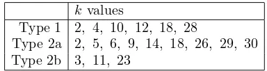
The optimal normal bases that are derived from the first part of the theorem are named Type 1, while the ones that follow from the second part are named Type 2 bases, or more specifically, as Type 2a and Type 2b bases. Fork≤30, the optimal normal bases are listed in Table 1.
Table 1:The optimal normal bases for k≤30.
kvalues
Type 1 2, 4, 10, 12, 18, 28
Type 2a 2, 5, 6, 9, 14, 18, 26, 29, 30 Type 2b 3, 11, 23
3
Normal Basis Multiplication Algorithm
Given the input operandsaandbas
a= k−1 X
i=0
aiβi , b= k−1 X
i=0 biβi ,
the multiplication algorithm computes each bit of the productc, which can be written as a double summation as
c= k−1 X
i=0
k−1 X
j=0
aibjβiβj .
This in turn can be written as a vector-matrix product
a0a1· · · ak−1λb0b1· · · bk−1
T
, (1)
such that every element of thek×kmatrixλis the sum of a subset of the normal elements {β0, β1, β2, . . . , βk−1}. Furthermore, theλ matrix can be expressed in
terms of thek×kmatricesλi fori= 0,1, . . . , k−1 with entries in {0,1}such that
λ=λ0β0+λ1β1+λ2β2+· · ·+λk−1βk−1 . (2)
4
Direct Multiplication in GF(2
2)
Consider the smallest extension field GF(22), which has both Type 1 and Type 2
of optimal normal bases. We will use the Type 1 optimal normal elementβ =x
and the irreducible polynomial p(x) = x2 +x+ 1, and derive the λ matrix.
Given the normal representations of two elements of the field a=a0β0+a1β1
andb=b0β0+b1β1, their productc is given as
c=a0b0β02+a0b1β0β1+a1b0β0β1+a1b1β21
where the equalities β2
0 =β1, β0β1=β0+β1, andβ21 =β0 are obtained using
the normal elementβ=xand the irreducible polynomialp(x) =x2+x+ 1. The
vector-matrix expansion of the product can be written as
c= a0a1
β1 β0+β1 β0+β1 β0
b0 b1
,
which gives us the λmatrix as
λ=
β1 β0+β1 β0+β1 β0
.
Furthermore, we obtain theλ0 andλ1 matrices for GF(22) as
λ=λ0β0+λ1β1=
β1 β0+β1 β0+β1 β0
= 0 1 1 1 β0 + 1 1 1 0 β1 .
Once all partial productsaibj for 0≤i, j ≤k−1 are computed usingk2 AND gates, the λi matrices determine which subsets of the partial productsaibj are to be summed to obtain a particular product termcr. For GF(22), we have
c0= a0a1 0 1 1 1 b0 b1
= a0b1+a1b0+a1b1 , (3)
c1= a0a1 1 1 1 0 b0 b1
= a0b0+a0b1+a1b0 . (4)
There are 3 1s in each of the λ0 andλ1 matrices, and therefore, there 3 terms
partial product terms aibj in the expressions forc0 or c1. The total number of XOR gates to compute both ofc0andc1is 2·2 = 4.
5
Matrix Decomposition Method for GF(2
2)
However, we observe a certain similarity in the λ0 and λ1 matrices: each can
be written as the sum of two matrices such that the first matrix is the same for both, in other words,
λ0=
0 1 1 1 = 0 1 1 0 + 0 0 0 1 , (5)
λ1=
1 1 1 0 = 0 1 1 0 + 1 0 0 0 . (6)
This matrix decomposition implies that the computation of c0 and c1 can be performed in two steps: the first step involves a common matrix for bothc0and
c1, and while the second steps involve two different matrices.
The first vector-matrix product needs to be performed only once for both c0
andc1, followed by the second vector-matrix products which need to performed separately for eachc0andc1. After these steps, we need add the partial sums to getc0 andc1. Therefore, our algorithm for GF(22) follows the following steps:
– Step 1: First, we compute the common partial product term, which requires one XOR gate and oneTX delay:
s= a0a1
0 1 1 0
b0 b1
=a0b1+a1b0. (7)
– Step 2: Now, we use the decomposition ofλ0 andλ1 to computet0 andt1;
this step does not require any XOR gates and any delay:
t0= a0a1
0 0 0 1
b0 b1
=a1b1 , (8)
t1= a0a1
1 0 0 0
b0 b1
=a0b0 . (9)
– Step 3: Finally we computec0andc1 usingc0=s+t0andc1=s+t1. This step requires one XOR gate and oneTX delay.
The matrix decomposition method for GF(22) reduces the number of XOR gates
to 3, while the direct computation using the formulae (3) and (4) imply 4 XOR gates. The total gate delay isTA+ 2TX.
6
Matrix Decomposition Method for GF(2
4)
The success of the decomposition method in GF(2k) depends on the the additive components the λi matrices, i.e., whether they have common terms among the expressions forcr. We now consider the field GF(24) with the Type 1 optimal normal basis β = x3 and the irreducible polynomial p(x) = x4+x+ 1. The
normal representations of the powers of β can be obtained by powering β and reducing the resulting polynomials mod p(x), as shown in [1]. The resulting λ
matrix is
λ=
β2 β3 β5 β9 β3 β4 β6 β10 β5 β6 β8 β12 β9β10β12β16
=
β1β3 1 β2 β3β2β0 1
1 β0β3β1 β2 1 β1β0
.
The number of terms in theλmatrix for the optimal basisβ ∈GF(24) is equal to
4·(2·4−1) = 28. This implies 4·(2·4−2) = 24 XOR gates in direct computation of the normal basis multiplication. To apply the matrix decomposition method, similar to the case of GF(22), we first derive the 4×4λ
the decomposition of theλi matrices as follows:
λ0=
0 0 1 0 0 0 1 1 1 1 0 0 0 1 0 1
=
0 0 1 0 0 0 0 1 1 0 0 0 0 1 0 0
+
0 0 0 0 0 0 1 0 0 1 0 0 0 0 0 1
, (10)
λ1=
1 0 1 0 0 0 0 1 1 0 0 1 0 1 1 0
=
0 0 1 0 0 0 0 1 1 0 0 0 0 1 0 0
+
1 0 0 0 0 0 0 0 0 0 0 1 0 0 1 0
, (11)
λ2=
0 0 1 1 0 1 0 1 1 0 0 1 1 1 1 0
=
0 0 1 0 0 0 0 1 1 0 0 0 0 1 0 0
+
0 0 0 1 0 1 0 0 0 0 0 0 1 0 0 0
, (12)
λ3=
0 1 1 0 1 0 0 1 1 0 1 0 0 1 0 0
=
0 0 1 0 0 0 0 1 1 0 0 0 0 1 0 0
+
0 1 0 0 1 0 0 0 0 0 1 0 0 0 0 0
. (13)
The steps of our algorithm for the normal basis multiplication in GF(24) are:
– Step 1: First, we compute the common partial product term using 3 XOR gates. This step requires 2TXgate delays, by arranging the sum computation as a binary tree with 4 leaves, with depth 2TX.
s=
a0a1a2a3
0 0 1 0 0 0 0 1 1 0 0 0 0 1 0 0
b0 b1 b2 b3
=a0b2+a1b3+a2b0+a3b1 . (14)
– Step 2: Then, we use the decomposition of λi to compute all 4 tr terms 4×2 = 8 XOR gates. This step also requires 2TX gate delays.
t0=
a0a1a2a3
0 0 0 0 0 0 1 0 0 1 0 0 0 0 0 1
b0 b1 b2 b3
=a2b1+a1b2+a3b3, (15)
t1=
a0a1a2a3
1 0 0 0 0 0 0 0 0 0 0 1 0 0 1 0
b0 b1 b2 b3
=a0b0+a3b2+a2b3, (16)
t2=
a0a1a2a3
0 0 0 1 0 1 0 0 0 0 0 0 1 0 0 0
b0 b1 b2 b3
t3=
a0a1a2a3
0 1 0 0 1 0 0 0 0 0 1 0 0 0 0 0
b0 b1 b2 b3
=a1b0+a0b1+a2b2. (18)
– Step 3: Finally, we computecrforr= 0,1,2,3 using 4 XOR gates:cr=s+tr. This will require a singleTX gate delay.
The computation ofc0, c1, c2, c3using the matrix decomposition method requires 3 + 8 + 4 = 15 XOR gates, instead 24 XOR gates required by the direct method. Since Steps 1 and 2 are independent of one another, the total gate delay is equal toTA+ 3TX.
7
Decomposition Method for Type 1 Bases in GF(2
k)
The decomposition method reduces the number of XOR gates due to the common partial product terms aibj among the computation of cr terms. We define the intersection of two or more λr matrices as the matrix whose (i, j) element is 1 if all input matricesλr has a 1 in their (i, j) location, and 0 otherwise. The intersection of allλrmatrices is the matrix used the computation of the partial product terms. We will denote this matrix byµ; for GF(22) we obtained it as
µ=λ0
\
λ1=
0 1 1 1
\1 1
1 0 = 0 1 1 0 ,
Similarly, we obtained theµmatrix for GF(24) as
µ=
3 \
r=0
λr=
0 0 1 0 0 0 1 1 1 1 0 0 0 1 0 1
\
1 0 1 0 0 0 0 1 1 0 0 1 0 1 1 0
\
0 0 1 1 0 1 0 1 1 0 0 1 1 1 1 0
\
0 1 1 0 1 0 0 1 1 0 1 0 0 1 0 0
=
0 0 1 0 0 0 0 1 1 0 0 0 0 1 0 0
.
Once the µ matrix is available, any ofλr matrices for r = 0,1, . . . , k−1 can be written in terms ofµand a second matrix. Let us denote the second matrix with νr in the computation of tr for GF(2k). Thus, we haveµ=Tkr−=01λr and
λr=µ+νr forr= 0,1, . . . , k−1.
Of course, it is possible that the µmatrix can be a zero matrix, implying that there are no common 1s among allλr matrices. In this case, our method would reduce to the direct method, not offering any savings in the number of XOR gates:λr=νr.
1. First, we construct the λ matrix. The (i, j) entry of λ matrix is equal to
β2i+2j
for 0≤i, j≤k−1, whereβ is the normal element. 2. We express β2i+2j
in the normal basis, i.e., express it as a linear sum of power of two powers ofβ. Thus, we obtain the λ matrix expressed in the normal basis. This can be accomplished using the polynomial representation ofβ and the irreducible polynomial of the field to obtain all non-power of 2 powers ofβ in the normal basis.
3. We obtain theλrmatrices forr= 0,1, . . . , k−1 by expanding theλmatrix as a linear sum of the basis elementsβr.
4. We obtain the intersection matrixµ=Tk−1
r=0λr.
5. Each νr matrix is then obtained usingνr=λr−µfori= 0,1, . . . , k−1.
The construction ofµandνrmatrices depend on the number common 1s in the
λrmatrices, which in turn depend on the structure and entries of theλmatrix. In order to analyze the complexity of the new multiplication algorithm, we need to look into the properties of theλmatrix.
Let us assume that GF(2k) has a Type 1 optimal normal basis; this implies that k+ 1 is prime and 2 is primitive in Z∗
k+1. Moreover, the optimal normal
element β is a primitive (k+ 1)st root of 1 in GF(2k). We writek = 2m and use B to represent the basis set B={β0, β1, . . . , βk−1}. The (i, j) entry of the
matrixλfor 0≤i, j≤k−1 is given as
λij =β2
i+2j
=β2iβ2j =βiβj .
Now we refer to Lemmas 1 and 2 in [1] about the structure of theλmatrix. The proofs are also given in the same article; we note that the proofs do not assume a particular type of irreducible polynomial generating the field GF(2k).
Lemma 1. The elements ofλwith the indices(i, i+mmodk)fori= 0,1, . . . , k−
1 are all 1s, where 1=β0+β1+· · ·+βk−1 andm=k/2.
Lemma 2. The rowrfor 0≤r≤k−1ofλis a permutation of B − {βr} with
1appearing in the column index m+r modk.
We will denote the set of indices for which the elements ofλare all1s byLas
L={(i, i+mmodk)| i= 0,1,2, . . . , k−1}.
Note thatLhask elements. As an example, fork= 10,Lis obtained as
which is seen in the λmatrix for GF(210) below: λ=
β1β8β4β6β9 1 β5β3β2β7 β8β2β9β5β7β0 1 β6β4β3 β4β9β3β0β6β8β1 1 β7β5 β6β5β0β4β1β7β9β2 1 β8 β9β7β6β1β5β2β8β0β3 1 1 β0β8β7β2β6β3β9β1β4 β5 1 β1β9β8β3β7β4β0β2 β3β6 1 β2β0β9β4β8β5β1 β2β4β7 1 β3β1β0β5β9β6 β7β3β5β8 1 β4β2β1β6β0 .
Using Lemmas 1 and 2, we will prove the following theorem.
Theorem 2. The λr matrix of the field GF(2k) with a Type 1 basis can be written as the sum of two matricesµandνrsuch that elements of the µmatrix with indices in the set L={(i, i+mmodk) |i= 0,1,2, . . . , k−1} are 1s. All other entries of µ are zero. Furthermore, the νr matrix hask−1 1s such that the rowr is all zero and every other row has a single 1.
Proof. Since the entries of λ with indices in set L are all1(which is equal to the sum of allkbasis elements), the entries of allλrmatrices with indices in the set L will be 1. Since the µmatrix is equal to the intersection of λr matrices, such entries ofµwill be equal to 1 as well. Furthermore, consider an entry ofλ
matrix with index (i, j)6∈L. This entry would not be equal to1, thus, missing at least one basis element. This implies a zero in the (i, j)6∈Llocation of one of theλrmatrices, and therefore, a zero in the intersection of all of them, which is theµmatrix. Therefore, the (i, j) entry of theµmatrix will be 1 iff (i, j)∈L
and 0 otherwise.
On the other hand we obtainedνrmatrices by subtractingµfromλr, how-ever, equivalently they can be computed from theλmatrix by first removing1s, and then expanding the resulting matrix (which will be denoted byλ′) in terms of all basis elements. For example, for GF(24) we can obtainν
r matrices from theλ′ matrix by expanding it into a sum of all basis elements
λ′=ν0β0+ν1β1+ν2β2+ν3β3
such that λ′=
β1β3 0 β2 β3β2β0 0
0 β0β3β1 β2 0 β1β0 =
0 0 0 0 0 0 1 0 0 1 0 0 0 0 0 1
β0+
1 0 0 0 0 0 0 0 0 0 0 1 0 0 1 0
β1+
0 0 0 1 0 1 0 0 0 0 0 0 1 0 0 0
β2+
0 1 0 0 1 0 0 0 0 0 1 0 0 0 0 0
β3.
Due to Lemma 2, the rowrof theλ′matrix is a permutation of all basis elements
Theorem 3. The decomposition method for the Type 1 optimal normal basis in GF(2k)computes all product termsc
rforr= 0,1, . . . , k−1usingk2AND gates,
k2−1 XOR gates, and T
A+ [1 + log2(k)]TX delay.
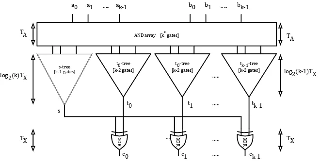
Proof. The common termsis computed using
s=
a0a1· · · ak−1 µ
b0 b1
.. .
bk−1
.
According to Theorem 2, the µmatrix has exactly k 1s with the indices inL, and all other terms are zero. This implies that we computesusing a linear sum which containsk terms:
s= k−1 X
i=0
aibi+mmodk .
The computation of s is accomplished using a binary tree of XOR gates with
k leaves; the number of XOR gates to computesis k−1, while the delay (the depth of tree) is log2(k)TX. Thes-tree is illustrated in Figure 1.
On the other hand, a singletr term is computed using
tr=a0a1· · · ak−1 νr
b0 b1
.. .
bk−1
.
Also according to Theorem 2, the row r of the νr matrix is zero, while every other row has a single 1 in it. This implies that we computetrusing a sum which containsk−1 terms:
k−1 X
i=0
i6=r
aπibi=aπ0b0+· · ·+aπr−1br−1+aπr+1br+1+· · ·aπk−1bk−1 ,
where π is a permutation of the indices {0,1, . . . , r−1, r+ 1, . . . , k−1}. We create k identical binary trees of XOR gates, each of which has k−1 leaves, as shown in Figure 1, named as tr-trees. The computation of a single tr term requiresk−2 XOR gates and log2(k−1)TX delay. The parallel computation of alltr terms forr= 0,1, . . . , k−1 requiresk(k−2) XOR gates.
Once s and tr for alli = 0,1, . . . , k−1 are computed, the computation of a single product term cr requires one XOR gate and all product terms cr for
i= 0,1, . . . , k−1 requirekXOR gates. However we only need oneTX delay for this computation. Therefore, the total number of gates and the required delay are found as:
2. The computation oftrfor allr= 0,1, . . . , k−1 requiresk(k−2) XOR gates and log2(k−1)TX delay.
3. However, we should note that, as illustrated in Figure 1, the computation of
sandtr values are independent of one another. By arranging thes-tree and
tr-trees in parallel, we find the critical path length as log2(k)TX.
4. The computation of cr for allr= 0,1, . . . , k−1 requires kXOR gates and a singleTX delay.
Thus we find that the total number of the XOR gates required by the matrix decomposition method ask−1 +k(k−2) +k=k2−1, while the total delay is TA+ [1 + log2(k)]TX.
!"#$%&&%'$$$$()*$+%,-./
%0 %2 455 %)32 10 12 455 1)32
.3,&--()32$+%,-./
,03,&--()36$+%,-./ 78+69)32:;<
78+69):;<
,0 ,)32
455
.
,)323,&--()36$+%,-./
;!
=0 =)32
455
<
>
?
<
>
? ;<
;!
;<
,03,&--()36$+%,-./
=2
<
>
?
,2
455 455
455
Figure 1:The matrix decomposition method for Type 1 basis.
8
Decomposition for Type 2a Bases in GF(2
k)
We now analyze the complexity of the decomposition algorithm for Type 2a bases. We will first derive the λ matrix for the field GF(25), which has Type
2a basis since p= 2k+ 1 = 11 is prime and 2 is primitive mod 11. Theorem 1 states that the basis elementβ can be written asβ =γ+γ−1such thatγis the
11th root of identity. Our objective is to discover how the λr matrices can be additively decomposed. Theλmatrix is given as
λ=
β2 β3 β5 β9 β17 β3 β4 β6 β10β18 β5 β6 β8 β12β20 β9 β10β12β16β24 β17β18β20β24β32
.
entries of theλmatrix which already contains powers of 2 powers ofβ. We have
βr =β2
r
for r= 0,1,2,3,4, and alsoβ32 =β =β0. Moreover we should also
note thatβ0=β=γ+γ−1, and
βr=β2
r
= (γ+γ−1)2r
=γ2r
+γ−2r
for r = 0,1,2,3,4. Next we obtain the normal expansions of the off-diagonal entries which contain the products of two basis elements β2i
·β2j
for i, j = 0,1,2,3,4 andi6=j. For example, the termβ21
·β23
=β10is written
β2·β8= (γ2+γ−2)(γ8+γ−8)
=γ10+γ−10+γ6+γ−6
which contains 10,−10,6,−6 powers of γ. We need to express these powers of
γ in terms of the powers of 2 powers of γ, and thus obtain a normal expansion for β10. In order to accomplish this, we will use Theorem 1. The general form
an off-diagonal product term is written as
β2i+2j =γ2i+2j +γ−2i
−2j
+γ2i−2j
+γ−2i+2j
for 0≤i, j≤4 andi6=j. By enumeratingiandj, we obtain the set of integers of the form±2i±2j as
±{1,2,3,4,5,6,7,8,9,10,12,14,15,17,18,20,24}.
In other words, we need the above powers ofγ in order to express allβ powers found in the λ matrix in the normal basis. Referring to the properties of the Type 2a basis in Theorem 1, we make the following observations:
– p= 2k+ 1 = 11 is prime.
– γ is 11th root of identity, implying that if u= v (mod 11) then γu =γv. Therefore, the above set is reduced mod 11, and we only need the powers of
γfrom the setZ∗
11={1,2,3,4,5,6,7,8,9,10}.
– 2 is primitive mod 11, that is, the powers of 2 generates the setZ∗
11. Since
210= 1 (mod 11) and 25=−1 (mod 11), which implies that 2u withu >5 can be written as 2u= 2v+5= 2v·25=−2v.
Thus, we can list elements ofZ∗
11as
20 21 22 23 24 25 26 27 28 29
1 2 4 8 5 10 9 7 3 6
20 21 22 23 24 −1 −21 −22 −23 −24
Thus, anyu∈ Z∗
11 can be written asu=±2v (mod 11) for av∈ {0,1,2,3,4}.
This implies that we can writeγu=γ±2v
for anyu∈ Z∗
11andv∈ {0,1,2,3,4}.
Table 2:The powers ofγ equalities.
u u (mod 11) u=±2v (mod 11) γ expansion
3 3 3 =−23 γ3=γ−23
5 5 5 = 24 γ5=γ24
6 6 6 =−24 γ6=γ−24
7 7 7 =−22 γ7=γ−22
9 9 9 =−21 γ9=γ−2
10 10 10 =−20 γ10=γ−1
12 1 1 = 20 γ12=γ
14 3 3 =−23 γ14=γ−23
15 4 4 = 22 γ15=γ22
17 6 6 =−24 γ17=γ−24
18 7 7 =−22 γ7=γ−22
20 9 9 =−21 γ20=γ−2
24 2 2 = 21 γ24=γ2
Thus, given the equalities γ10 = γ−1 and γ6 = γ−24
, we obtain the normal expansion of the productβ10as
β2·β8=γ10+γ−10+γ6+γ−6
=γ−1+γ+γ−24+γ24
=β0+β4.
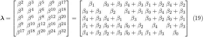
The other powers ofβ can be obtained using similar derivations. We omit these derivations, and write theλmatrix for GF(25) below.
λ=
β2 β3 β5 β9 β17 β3 β4 β6 β10β18 β5 β6 β8 β12β20 β9 β10β12β16β24 β17β18β20β24β32
=
β1 β0+β3β4+β3β1+β2β4+β2 β0+β3 β2 β4+β1β0+β4β2+β3 β4+β3β4+β1 β3 β0+β2β0+β1 β1+β2β0+β4β0+β2 β4 β1+β3 β4+β2β2+β3β0+β1β1+β3 β0
(19)
We observe that the λ matrix for GF(25) does not have any 1 entries, and
therefore, the intersection of all λr matrices is a zero matrix. Unfortunately, a decomposition as in the Type 1 case (which was of the formλr=µ+νr) is not possible. However, we will show that another decomposition exists.
Theorem 4. The diagonal entries of theλ matrix for the field GF(2k)with a Type 2a basis contain one basis element, while all other entries are the sum of two basis elements.
Proof. The normal elementβ of the field GF(2k) with a Type 2a basis is given as β =γ+γ−1 where p= 2k+ 1 is prime, 2 is primitive modp, andγ is the
First we observe that all diagonal elements are of the form β2r
for r = 0,1, . . . , k−1, therefore, each contains a single basis element β2r
=βr forr= 1,2, . . . , k−1 andβ2k
=β=β0forr=k. Moreoverβr=β2
r
=γ2r
+γ−2r
for
r= 0,1, . . . , k−1.
Now consider the (i, j) element of theλfor 0≤i, j≤k−1 andi6=j. This elementβ2i+2j
is a product and can be written as
β2i·β2j = (γ2i+γ−2i)(γ2j +γ−2j) =γ2i+2j +γ−(2i+2j)
+γ2i−2j
+γ−(2i
−2j)
,
Since γp is the identity, the powers of γ above can be reduced mod p, and therefore, we can write
β2i+2j =γu1+γ−u1+γu2+γ−u2 , (20)
such thatu1= 2i+ 2j (mod p) andu2= 2i−2j (modp), where 0≤i, j≤k−1 and i 6=j. Now we will prove that any integeru∈ Z∗
p = {1,2, . . . , p−1} can be uniquely written as u= ±2v (mod p) for some v ∈ Z
k ={0,1, . . . , k−1}. Sincep= 2k+ 1 prime and 2 is primitive modp, we have 22k= 1 (mod p) and 2k =−1 (modp). Thus, we can generate all elements ofZ∗
p using powers of 2, and furthermore, using the identity 2k=−1 (modp) we obtain
Zp∗={20,21,22, . . . ,2k−1,2k,2k+1,2k+2, . . . ,22k−1}
={20,21,22, . . . ,2k−1,−1,−21,−22, . . . ,−2k−1}.
This implies that anyu∈ Z∗
p can be written asu=±2v (mod p) withv∈ Zk. Thus, we conclude thatγu=γ±2v
, and write Eqn. (22) as
β2i+2j =γ2v1
+γ−2v1
+γ2v2
+γ−2v2 ,
Therefore, every off-diagonal element of theλmatrix constructed using Type 2a normal basis of the field GF(2k) contains the sum of 2 basis elements.
In order to decomposeλrmatrices, we will first separate the diagonal entries and place each of them in different matrices for eachr, which we denote asµr. As the off-diagonal entries are concerned, we notice that theλmatrix is symmet-ric, implying these pairs of elements appear in two different (and symmetrical) locations. For example,β0+β1is in the locations (2,4) and (4,2) of theλmatrix for GF(25). Since λ
0 and λ1 matrices respectively hold the coefficients of the
basis elements β0 and β1, these matrices would have 1s in the same locations (2,4) and (4,2), and thus, their intersection would be a nonzero matrix. Fur-thermore, β0 is coupled with every other βr, the intersection ofλ0 withλr for
Theorem 5. The λr matrix for the field GF(2k) with a Type 2a basis can be written as the sum of kmatrices such that
λr=µr+
k−1 X
i=0
i6=r
νri ,
where each µr matrix has a single 1 in location (k−1, k−1) for r = 0 and (r−1, r−1)for r= 1,2, . . . , k−1. Furthermore, eachνri matrix is symmetric and contains only two 1s.
Proof. Theµr matrix contains only the diagonal entries ofλrmatrix. As illus-trated for GF(25) in Eqn. (19) the diagonal entries of theλmatrix has the basis
elementsβrforr= 1,2, . . . , k−1,0.
β1 β0+β3β4+β3β1+β2β4+β2 β0+β3 β2 β4+β1β0+β4β2+β3 β4+β3β4+β1 β3 β0+β2β0+β1 β1+β2β0+β4β0+β2 β4 β1+β3 β4+β2β2+β3β0+β1β1+β3 β0
.
Therefore, the diagonal of theλr matrix has a single 1, and thus, the entireµr matrix has only 1 in it; all remaining elements are 0. The µ0 matrix has a 1
in the location (k−1, k−1) while µr has a 1 in the location (r−1, r−1) for
r= 1,2, . . . , k−1. We obtain theλr matrices as
λ0 λ1 λ2 λ3 λ4
0 1 0 0 0 1 0 0 1 0 0 0 0 1 1 0 1 1 0 0 0 0 1 0 1
1 0 0 1 0 0 0 1 0 0 0 1 0 0 1 1 0 0 0 1 0 0 1 1 0
0 0 0 1 1 0 1 0 0 1 0 0 0 1 0 1 0 1 0 0 1 1 0 0 0
0 1 1 0 0 1 0 0 0 1 1 0 1 0 0 0 0 0 0 1 0 1 0 1 0
0 0 1 0 1 0 0 1 1 0 1 1 0 0 0 0 1 0 1 0 1 0 0 0 0
Furthermore, we obtain theµrmatrices as follows:
µ0 µ1 µ2 µ3 µ4
0 0 0 0 0 0 0 0 0 0 0 0 0 0 0 0 0 0 0 0 0 0 0 0 1
1 0 0 0 0 0 0 0 0 0 0 0 0 0 0 0 0 0 0 0 0 0 0 0 0
0 0 0 0 0 0 1 0 0 0 0 0 0 0 0 0 0 0 0 0 0 0 0 0 0
0 0 0 0 0 0 0 0 0 0 0 0 1 0 0 0 0 0 0 0 0 0 0 0 0
0 0 0 0 0 0 0 0 0 0 0 0 0 0 0 0 0 0 1 0 0 0 0 0 0
We denote the matrix asνri as the intersection of theλr andλi matrices as
νri=λr
\
λi for r6=i .
matrix contains only two 1s, and all other elements are zero. For example,ν0i matrices for GF(25) are obtained as
ν01 ν02 ν03 ν04
0 0 0 0 0 0 0 0 0 0 0 0 0 0 1 0 0 0 0 0 0 0 1 0 0
0 0 0 0 0 0 0 0 0 0 0 0 0 1 0 0 0 1 0 0 0 0 0 0 0
0 1 0 0 0 1 0 0 0 0 0 0 0 0 0 0 0 0 0 0 0 0 0 0 0
0 0 0 0 0 0 0 0 1 0 0 0 0 0 0 0 1 0 0 0 0 0 0 0 0
Therefore, theλr matrix of GF(2k) decomposes intokmatrices µr andνri for
i= 0,1, . . . , r−1, r+ 1, . . . , k−1 such that the µr matrix contains a single 1, and allνrimatrices contain 2 1s.
The space complexity of the multiplication using decomposition method is ana-lyzed in the following theorem.
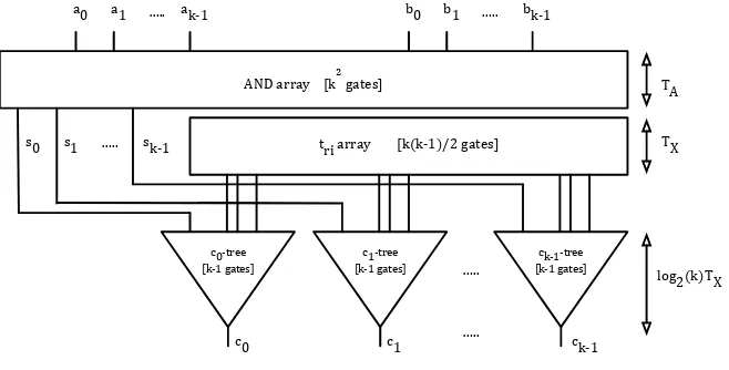
Theorem 6. The decomposition method for the Type 2a optimal normal basis in GF(2k) computes all product terms c
r for r= 0,1, . . . , k−1 using k2 AND gates, 1.5k(k−1) XOR gates, and a total delay ofTA+ [1 + log2(k)]TX.
Proof. According to Theorem 5, the λr matrix can be written as the sum of k matrices as
λr=µr+
k−1 X
i=0
i6=r
νri .
The computation of the product termcr is accomplished using
cr=
a0a1· · · ak−1
µr+
k−1 X
i=0
i6=r
νri b0 b1 .. .
bk−1 .
For brevity, we will denote the input vectors byaT andb, and break the above product computation into the sum ofkmatrix-vector products as
cr=aT µrb+ k−1 X
i=0
i6=r
aT νri b=sr+
k−1 X
i=0
i6=r
tri . (21)
The individual components of the above sum,sr andtri, are defined as
sr=aT µr b,
tri=aT νri b,
1. The computation ofsrdoes not require any XOR gates. The matrixµrhas a single 1 in it; the location is (k−1, k−1) forr= 0 and (r−1, r−1) for all otherr = 1,2, . . . , k−1. Therefore, s0 =ak−1bk−1 and sr = ar−1br−1
forr= 1,2, . . . , k−1. There is no delay involved, either, the selection logic works by routing the logic signals.
2. Theνri has only two 1s and it is also symmetric. If the (u, v) element of the
νrimatrix is 1, then so is (v, u) element, while all the other elements are zero. This gives the value oftri as aubv+avbu. Therefore, the computation of a singletrirequires 1 XOR gate andTXdelay. Furthermore, we haveνri=νir, and thus,tri =tir. This implies that we only need to compute half of the
tir terms due to the symmetry. For example, for k= 5 the following terms need to be computed:t0i fori= 1,2,3,4;t1i for i= 2,3,4;t2i for i= 3,4; finallyt34. For GF(2k) the number of terms that need to be computed is
(k−1) + (k−2) +· · ·+ 1 =k(k−1)/2,
which gives the total number of XOR gates for computing alltri terms as 0.5k(k−1), while the delay is still equal to oneTX.
3. Having obtained all sr andtri values, we computecr using the summation Eqn. (21) which haskterms. We arrange this summation using a binary tree of XOR gates, which hask leaves. There is a separate binary for each value ofr= 0,1, . . . , k−1; there arekinputs for each tree such thatsr, triexcept
trr term. The computation of a singlecr term requiresk−1 XOR gates and log2(k)TX units of delay, while allcrterms would require a total ofk(k−1) XOR gates.
Therefore the total number of XOR gates is found as 1.5k(k−1), and the total delay isTA+ [1 + log2(k)]TX.
!"#$%&&%'$$$$()*$+%,-./
%0 %2 455 %)32 10 12 455 1)32
67+89):;< 455
;!
.0 .2 455 .)32 ,&=$%&&%'$$$$$$$$()9)32:>8$+%,-./
?)323,&--()32$+%,-./
?03,&--()32$+%,-./
?23,&--()32$+%,-./
?0 ?2 455 ?)32
;<
9
Decomposition for Type 2b Bases in GF(2
k)
The smallest field with the Type 2b basis is GF(23). For k = 3, we have p=
2k+ 1 = 7 prime,p= 3 (mod 4), and 2 generates the quadratic residues inZ∗
7.
Furthermore, a basis elementβi=β2
i
is equal toγ2i
+γ−2i
fori= 0,1,2, where
γ is the 7th root of identity according to Theorem 1. We can write γ3 =γ−4, γ5=γ−2, andγ6=γ−1, and obtain the products of the basis elements as
ββ2=β3=γ3+γ−3+γ+γ−1
=γ−4+γ4+γ+γ−1
=β0+β2
ββ4=β5=γ5+γ−5+γ3+γ−3
=γ−2+γ2+γ4+γ−4
=β1+β2
β2β4=β6=γ6+γ−6+γ2+γ−2
=γ−1+γ+γ2+γ−2
=β0+β1
Therefore, the λmatrix is obtained as
λ=
β2β3β5 β3β4β6 β5β6β8
=
β1 β0+β2β1+β2 β0+β2 β2 β0+β1 β1+β2β0+β1 β0
.
Similar to the Type 2a case, we see that the λ matrix for GF(23) contains a
single basis on the diagonal, while all off-diagonal elements are equal to and the sum of two bases. We prove that this property holds true for anyk.
Theorem 7. The diagonal entries of theλ matrix for the field GF(2k)with a Type 2b basis contain one basis element, while all other entries are the sum of two basis elements.
Proof. All diagonal elements of theλmatrix are of the formβ2r
, and therefore, each contains a single basis elementβ2r
=βrfor 0 = 1,2, . . . , k−1. Furthermore, we have β = γ+γ−1 where γ is the p = 2k+ 1 primitive root of identity. A
diagonal element is of the formβ2r
=γ2r
+γ−2r
forr= 0,1, . . . , k−1. Similar to the Type 2a case, an off-diagonal element is given as β2i+2j
for
i= 1,2, . . . , j−1, j+ 1, . . . , k−1, which is equal to
β2i·β2j =γ2i+2j +γ−(2i+2j)
+γ2i−2j
+γ−(2i
−2j)
.
Sinceγpis the identity, the powers ofγabove are reduced modp, and therefore, we can write
such thatu1= 2i+ 2j (mod p) andu2= 2i−2j (modp), where 0≤i, j≤k−1 andi6=j. Next we will prove that any integeru∈ Z∗
p ={1,2, . . . , p−1}can be uniquely written asu=±2v (modp) for somev∈ Z
k={0,1, . . . , k−1}. Theorem 1 states that for Type 2b basis, p = 3 (mod 4) and 2 generates quadratic residues mod p. We use Qp to denote the set of quadratic residues, which has (p−1)/2 elements. An elementu∈ Z∗
p is inQp if there is a solution
xfor the equation x2=u (modp), otherwiseuis a quadratic nonresidue. The
set of quadratic nonresidues, denoted byQ′
p, consists of the remaining (p−1)/2 elements ofZ∗
p. For example, fork= 11,p= 23, these two sets are given as
Q23={1,2,3,4,6,8,9,12,13,16,18}, Q′23={5,7,10,11,14,15,17,19,20,21,22}.
The Euler criterion determines ifu∈Qp oru∈Q′p:
u(p−1)/2= 1 if u∈Qp,
−1 if u∈Q′
p.
An important observation is that−1∈Q′
p ifp= 3 (mod 4), since
(−1)(p−1)/2=
1 if p= 1 (mod 4),
−1 if p= 3 (mod 4).
Another relevant property of quadratic residues is that if u ∈Qp and v ∈Q′p then the product uv ∈Q′
p. Particularly, in our case, we can write −u∈ Q′p if
u∈Qp, since−1∈Q′p. SinceQp is generated by powers of 2, it follows that
Qp={2v (mod p)|v∈ Zk}.
We can generateQ′
pby multiplying every element ofQp by−1, in other words,
Q′p={−2v (mod p)|v∈ Zk} .
SinceZ∗
p =QpSQ′p, we can write
Z∗
p ={±2v (mod p)|v∈ Zk} .
This implies that anyu∈ Z∗
p can be written asu=±2v (mod p) withv∈ Zk. Thus, we conclude thatγu=γ±2v
, and write Eqn. (22) as
β2i+2j =γ2v1
+γ−2v1
+γ2v2
+γ−2v2 ,
Therefore, every off-diagonal element of theλmatrix constructed using Type 2a normal basis of the field GF(2k) contains the sum of 2 basis elements.
Therefore, the same complexity analysis for Type 2a applies for Type 2b as well. The complexity of the multiplication using decomposition method for the Type 2b bases is the same as that of Type 2a bases.
10
Conclusions
We introduced a matrix decomposition method and described the underlying algorithms for normal basis multiplication in the field GF(2k) with Type 1 and Type 2 bases. The decomposition algorithm computes all product terms for the Type 1 basis usingk2−1 XOR gates, irrespective of the irreducible polynomial
generating the field. The previous Massey-Omura multiplication algorithms [5, 7, 14] accomplished the same bound using all-one-polynomials. Furthermore, our matrix decomposition algorithm computes all product terms for the Type 2a and 2b bases using 1.5k(k−1) XOR gates, which matches previous bounds [16, 14]. The Type 1 normal basis multiplication algorithm given in [14] is also based on a matrix decomposition in which theλmatrix is decomposed into upper and lower triangular matrices and a diagonal matrix. The XOR complexity of this algorithm is given for all-one-polynomials as k2−1, however, an analysis for
a general irreducible polynomial is not given. Instead, it was shown that the algorithm for GF(25) requires 8 XOR gates. However, one has to note that this
is a straightforward decomposition which follows directly the definition of sym-metric matrices, and separates the multiplication terms into three groups. Their algorithm then rearranges the terms of this sum. In our approach however, We find an optimal decomposition with respect to the chosen normal basis and the corresponding multiplication matrix. After creating the optimal decomposition we are able to create the circuit without any intermediate steps. For the opti-mal noropti-mal basism our results match the results in [14], but we do not restrict our algorithm to all-one polynomials, and we extends to arbitrary normal bases without additional effort.
It is also interesting to note that the Mastrovito algorithms, which work only for the polynomial basis, achieve the k2−1 space complexity with irreducible
trinomials [8, 9, 12, 13]. Furthermore, the space complexity falls to k2−∆ for
equally-spaced polynomials [15, 4], where∆is the distance factor; in other words, the irreducible polynomial is of the form
p(x) =xm∆+x(m−1)∆+· · ·+x∆+ 1 .
In a highly special case of equally-spaced-trinomial xk +xk/2+ 1, the space
complexity becomes k2−k/2 [15]. This implies that the bound k2−1 is not
very tight and there may be more special cases in which the space complexity falls further from that. However, it is highly likely that the result of this paper provides the lower bound for optimal normal bases, irrespective of the irreducible polynomial. This remains to be proven.
An interesting direction for future work is to investigate if we can reduce the space complexity for non-optimal (Gaussian) normal basis multiplication using our matrix decomposition approach.
References
LNCS Nr. 9061, Springer (2014)
2. Gao, S.: Normal Bases over Finite Fields. Ph.D. thesis, University of Waterloo (1993)
3. Gao, S., Lenstra, Jr., H.W.: Optimal normal bases. Designs, Codes and Cryptog-raphy 2(4), 315–323 (Dec 1992)
4. Halbutoˇgulları, A., Ko¸c, C¸ .K.: Mastrovito multiplier for general irreducible poly-nomials. IEEE Transactions on Computers 49(5), 503–518 (May 2000)
5. Hasan, M.A., Wang, M.Z., Bhargava, V.K.: Modular construction of low complex-ity parallel multipliers for a class of finite fields GF(2m
). IEEE Transactions on Computers 41(8), 962–971 (Aug 1992)
6. Hasan, M.A., Wang, M.Z., Bhargava, V.K.: A modified Massey-Omura parallel multiplier for a class of finite fields. IEEE Transactions on Computers 42(10), 1278–1280 (Nov 1993)
7. Ko¸c, C¸ .K., Sunar, B.: Low-complexity bit-parallel canonical and normal basis mul-tipliers for a class of finite fields. IEEE Transactions on Computers 47(3), 353–356 (Mar 1998)
8. Mastrovito, E.D.: VLSI architectures for multiplication over finite field GF(2m ). In: Mora, T. (ed.) Applied Algebra, Algebraic Algorithms and Error-Correcting Codes. pp. 297–309. Springer, LNCS Nr. 357 (1988)
9. Mastrovito, E.D.: VLSI Architectures for Computation in Galois Fields. Ph.D. the-sis, Link¨oping University, Department of Electrical Engineering, Link¨oping, Sweden (1991)
10. Mullin, R., Onyszchuk, I., Vanstone, S., Wilson, R.: Optimal normal bases in
GF(pn
). Discrete Applied Mathematics 22, 149–161 (1988)
11. Omura, J., Massey, J.: Computational method and apparatus for finite field arith-metic (May 1986), US Patent Number 4,587,627
12. Paar, C.: Efficient VLSI Architectures for Bit Parallel Computation in Galois Fields. Ph.D. thesis, Universit¨at GH Essen, VDI Verlag (1994)
13. Paar, C.: A new architecture for a paralel finite field multiplier with low complexity based on composite fields. IEEE Transactions on Computers 45(7), 856–861 (Jul 1996)
14. Reyhani-Masoleh, A., Hasan, M.A.: A new construction of Massey-Omura parallel multiplier over GF(2m
). IEEE Transactions on Computers 51(5), 511–520 (May 2002)
15. Sunar, B., Ko¸c, C¸ .K.: Mastrovito multiplier for all trinomials. IEEE Transactions on Computers 48(5), 522–527 (May 1999)