A Class of Estimators of Population Mean in Case of Post Stratification

(1)

A Class of Estimators of Population Mean

in Case of Post Stratification

Hilal A. Lone

School of Studies in Statistics

Vikram University, Ujjain-456010, M.P. India [email protected]

Rajesh Tailor

School of Studies in Statistics,

Vikram University, Ujjain-456010, M.P. India [email protected]

Abstract

This paper proposes a class of ratio-cum-product type estimators in case of post-stratification. Particular members of the proposed class of ratio-cum-product type estimators have been identified and studied thoroughly from efficiency point of view. It has been shown that the identified particular estimators are more efficient than the usual unbiased estimator, Ige and Tripathi (1989) estimators, Chouhan (2012) estimators, Tailor et al. (2016) estimator and other considered estimators. An empirical study has been carried out to demonstrate the performance of the proposed estimators.

Keywords: Mean squared error, Bias, Ratio-cum-product estimator.

1. Introduction

Cochran (1940) and Robson (1957) envisaged classical ratio and product estimators which were studied in case of post stratification by Ige and Tripathi (1989). Recently, Lone and Tailor (2014) and Lone and Tailor (2015) proposed ratio and product type exponential estimators in case of post-stratification. Chouhan (2012) proposed class of ratio type estimators using various known parameters of auxiliary variates in case of post stratification. Tailor et al. (2015) proposed dual to Ige and Tripathi (1989) ratio and product estimators. Tailor et al. (2016) proposed a ratio-cum-product type estimator in case of post-stratification. Singh (1967) used information on population mean of two auxiliary variates and proposed ratio-cum-product type estimator for population mean in simple random sampling. Singh (1967) and Chouhan (2012) motivate authors to propose the class of ratio-cum-product type estimators in case of post-stratification. Many Researchers including Holt and Smith (1979), Jagers et al. (1985), Jagers (1986), Ige and Tripathi (1989), Agrawal and Panday (1993), Singh and Ruiz Espejo (2003) Tailor et al. (2011) and Tailor et al. (2015) contributed well in case of post-stratification.

Let us consider a finite population U 



U₁,U₂,...,U_N



of size N_{which is divided into L} strata of size N₁,N₂,...,N_L such that N N

L

h h 



1

(2)

variate, negatively correlated with the study variate y. Let yhi be the observation on

th

i

unit of

h

th stratum for study variate y and x_hi and z_hi be the observation on

i

th unit of th

h

stratum for auxiliary variates x and

z

_{respectively, then}





 Nh

i hi h

h x

N X

1 1

: hth stratum mean for the auxiliary variate x,





 Nh

i hi h

h y

N Y

1 1

:hth stratum mean for the study variate y,





 Nh

i hi h

h x

N Z

1 1

: hth stratum mean for the auxiliary variate

z

,





  



 L

h

h h L

h N

i

hi W X

x N

X

h

1 1 1

1

: Population mean of the auxiliary variate x,





  



 L

h h h L

h N

i

hi W Y

y N

Y

h

1 1 1

1

: Population mean of the study variate y and





 L

h

h hZ

W Z

1

: Population mean of the auxiliary variate

z

.

A sample of size n_{is drawn from population}U _{using simple random sampling without} replacement. After selecting the sample, it is observed that which units belong to

h

th

stratum. Let n_h be the size of the sample falling in

h

th stratum such that n n

L

h h 



1

Here it is assumed that n is so large that possibility of n_h being zero is very small.

In case of post-stratification, usual unbiased estimator of population mean Y _{is defined} as





 L

h h h

PS W y

y

1

, (1.1)

where N N

W h

h  is the weight of the

th

h

stratum and





 nh

i hi h

h y

n y

1 1

is sample mean of n_h sample units that fall in the

h

th stratum.

Using the results from Stephen (1945), the variance of y_PS to the first degree of approximation is obtained as











 

 

   

  

 L

h

L

h

yh h yh

h

PS W S

n S W N n y

Var

1 1

2 2

2

1 1 1

1

(3)

where









 

 Nh

i

h hi h

yh y Y

N S

1

2 2

1 1

.

Ige and Tripathi (1989) defined a ratio and a product type estimator in case of post-stratification as

      

PS PS R PS

x X y

Yˆ (1.3)

and

      

Z z y

Y PS

PS P PS

ˆ _. _(1.4)

where





 L

h h h

PS W x

x

1

and





 L

h h h

PS W z

z 1

are the unbiased estimators of population means in case of post-stratification and x_h and z_h are the means of the samples of size n_h that in case of post-stratification and x_h and z_h are the means of the samples of size fall in hth stratum.

Mean squared error of the Ige and Tripathi (1989) estimators R PS

Yˆ and P PS

Yˆ are

 









 

   

  

 L

h

yxh xh

yh h R

PS W S R S RS

N n Y

MSE

1

1 2 2 1 2

2 1

1 ˆ

(1.5) and

 









 

   

  

 L

h

yzh zh

yh h P

PS W S R S R S

N n Y

MSE

1

2 2 2 2 2

2 1

1

ˆ _.

(1.6) where

X Y

R1 and

Z Y R2 .

Chouhan (2012) proposed the following ratio type estimators for population mean Y _in case of post-stratification as











 

 

   

 

  



 

xh h L

h h

xh h L

h h ps

RSD PS

C x W

C X W y

Y

1 1

ˆ _, _(1.7)











 

 

   

 

  



 

) (

) ( ˆ

2 1

x x

W

x X

W y

Y

h h L

h h

h h L

h h ps

RSE PS

 

(1.8)

(4)









             



  yxh h L h h yxh h L h h ps RST PS x W X W y Y   1 1

ˆ _, _(1.9)

Mean squared errors of the estimators Yˆ_PSRSD, Yˆ_PSRSE and Yˆ_PSRST upto the first degree of approximation are obtained as

 







           L h yxh n xh n yh h RSD

PS W S R S R S

N n Y MSE 1 1 2 2 1 2 2 1 1 ˆ _, (1.10)

 







           L h yxh n xh n yh h RSE

PS W S R S R S

N n Y MSE 1 2 2 2 2 2 2 1 1

ˆ _, _(1.11)

 







           L h yxh n xh n yh h RST

PS W S R S R S

N n Y MSE 1 3 2 2 3 2 2 1 1

ˆ _, _(1.12)

Where as the product version of RSD PS

Yˆ , RSE PS

Yˆ and RST PS

Yˆ can be written as









             



  zh h L h h zh h L h h ps PSD PS C Z W C z W y Y 1 1

ˆ _, _(1.13)









             



  L h h h h L h h h h ps PSE PS z Z W z z W y Y 1 2 1 2 ) ( ) ( ˆ   (1.14) and









             



  yzh h L h h yzh h L h h ps PST PS Z W z W y Y   1 1

ˆ _(1.15)

Upto the first degree of approximation, mean squared error of the estimators PSD PS

Yˆ , PSE PS

Yˆ

and Yˆ_PSPST are obtained as

 







           L h yzh m zh m yh h PSD

PS W S R S R S

N n Y MSE 1 1 2 2 1 2 2 1 1

ˆ _, _(1.16)

 







           L h yzh m zh m yh h PSE

PS W S R S R S

N n Y MSE 1 2 2 2 2 2 2 1 1

(5)

 







           L h yzh m zh m yh h PST

PS W S R S R S

N n Y MSE 1 3 2 2 3 2 2 1 1

ˆ _, _(1.18)

where

























. 3 / 2 ) ( / 1 / 3 / 2 ) ( / 1 / 1 2 1 1 1 2 1 1                                



      i Z W Y i z Z W Y i C Z W Y R and i X W Y i x X W Y i C X W Y R yzh h L h h h h L h h xh h L h h mi yxh h L h h h h L h h xh h L h h ni    

Tailor et al. (2016) proposed a ratio-cum-product type estimator in case of post-stratification as                         



    L h h h L h h h L h h h L h h h ps RP PS Z W z W x W X W y Y 1 1 1 1 ˆ _(1.19)

Up to the first degree of approximation, mean squared error of RP PS

Yˆ is obtained as

 











              L h yzh xzh yxh zh xh yh h RP

PS W S R S R S RS R R S R S

N n Y MSE 1 2 2 1 1 2 2 2 2 2 1 2 2 1 1 ˆ _(1.20)

2. Proposed Class of Ratio-Cum- Product Type Estimators

In the line of Singh (1967), we suggest a class of ratio-cum-product type estimators for estimating population mean Y _as

















                           



    L h h h h h L h h h h h L h h h h h L h h h h h ps d Z c W d z c W b x a W b X a W y t 1 1 1 1 (2.1)

where



a_h,b_h,c_hand d_h



are the function of population parameters of the auxiliary variates.

To obtain the bias and mean squared error of the proposed estimator t, we write



h



h

h Y e

y  1 ₀ , x_h  X_h



1e₁_h



and z_h Z_h



1e₂_h



such that 0 ) ( ) ( )

(e0h E e1h E e2h 

(6)

, 1 1 )

( 02 yh2

h h h C N nW e E _        2 2 1 1 1 ) ( _xh h h h C N nW e E _        , 2 2 2 1 1 ) ( zh h h h C N nW e E _        , xh yh yxh h h h

h C C

N nW e

e

E _

     

 1 1

)

( ₀ ₁ ,

zh yh yzh h h h

h C C

N nW e

e

E _

     

 1 1

)

( 0 2 and

zh xh xzh h h h

h C C

N nW e

e

E _

     

 1 1

)

( ₁ ₂ .

Expressing (2.1) in terms of e’s, we have

                                       



    m h h h L h h n h h h L h h h h L h h X e Z c W X e X a W Y e Y W Y t 2 1 1 1 1 0 1 1 1 1 ) 1 ( ) 1 ( ) 1

( e₀ e₁ 1 e₂ Y

t    



1 2 0 1 0 2



2 1 2 1

0 e e e ee e e e e

e Y Y

t       

 (2.2) where Y e Y W e h h L h h 0 1 0



  , n h h h L h h X e X a W e 1 1 1





 and

m h h h L h h X e Z c W e 2 1 2



  .

Taking expectation on both sides of (2.2), we get the bias of the proposed estimator t upto the first degree of approximation as

 

_         _        



  L h yxh h h n h L h xh h n S a W R a S W X N n t B 1 2 1 2 1 1 1          _ 



  L h xzh h h n h yzh h L h h m S c a R W S c W

X 1 1

1

(2.3)

(7)

 



n h yxh L

h

zh h m xh h n yh

h S R a S R c S R a S

W N n t

MSE 1 1 2

1

2 2 2 2 2 2

2   

   

  









yzh m h xzh h h m

n R a c S c R S

R 2

2 



(2.4) where

n n

X Y R  ,

m m

X Y

R  ,



_h _h _h



L

h h

n W a X b

X 





1

and



_h _h _h



L

h h

m W c Z d

X 





1

.

Equation (2.4) can also be written as

 

t A R B R C R D R R E R F

MSE   _n2  _m2 2 _n 2 _n _m 2 _m (2.5)

where





   

  

 L

h

yh hS

W N

n A

1 2

1 1

,





   

  

 L

h

xh h ha S

W N n B

1

2 2

1 1

,





   

  

 L

h

zh h hc S

W N n C

1

2 2

1 1

,





   

  

 L

h

yxh h ha S

W N n D

1

1 1

,





   

  

 L

h

xzh h h ha c S

W N n E

1

1 1

and





   

  

 L

h

yzh h hc S

W N n F

1

1 1

.

The MSE of t is minimum when

     

   

) (

) ( * 2

* 2

say R E BC

BF DE R

say R E BC

EF DC R

m m

n n

(2.6)

Putting (2.6) in (2.5), we get the minimum mean squared error of the proposed estimator t as

 





1





min t A

MSE (2.7)

where

) (

) 2 (

2 2 2

E BC A

DEF BF

CD

   

(8)

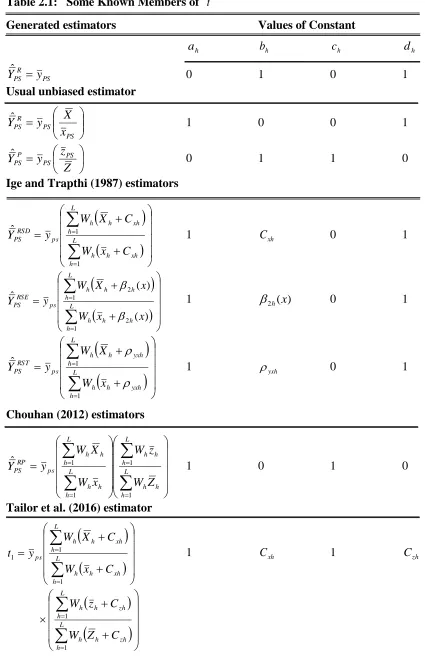
Table 2.1: Some Known Members of t

Generated estimators Values of Constant

h

a bh ch dh

PS R

PS y

Yˆ  0 1 0 1

Usual unbiased estimator

      

PS PS R PS

x X y

Yˆ 1 0 0 1

      

Z z y

Y PS

PS P PS

ˆ ₀ ₁ ₁ ₀

Ige and Trapthi (1987) estimators











 

 

   

 

  



 

xh h L

h h

xh h L

h h ps

RSD PS

C x W

C X W y

Y

1 1

ˆ ₁

xh

C 0 1











 

 

   

 

  



 

) (

) ( ˆ

2 1

x x

W

x X

W y

Y

h h L h

h

h h L

h h ps RSE PS

 

1 ₂_h(x) 0 1











 

 

   

 

  



 

yxh h L

h h

yxh h L

h h ps

RST PS

x W

X W y

Y

 

1 1

ˆ ₁

yxh

 0 1

Chouhan (2012) estimators

   

 

   

 

   

 

   

  



 

L

h

h h L

h h h L

h

h h ps

RP PS

Z W

z W

x W

X W y

Y

1 1 1

1

ˆ ₁ ₀ ₁ ₀

Tailor et al. (2016) estimator











 

 

   

 

  



 

xh h L

h h

xh h L

h h ps

C x W

C X W y

t

1 1

1 1 Cxh 1 Czh









  

 

   

 

  





zh h L

h

zh h L

h h

C Z W

C z W

(9)











 

 

   

 

  



 

L

h

h h h L

h

h h h ps

x x

W

x X

W y

t

1

2 1

2 2

) (

 

1 ₂_h(x) 1 ₂_h(z)











 

 

   

 

  



 

L

h

h h h L

h

h h h

z Z

W

z z

W

1

2 1

2

) (

 











 

 

   

 

  



 

yxh h L

h h

yxh h L

h h ps

x W

X W y

t

 

1 1

3 1 yxh 1 yzh











 

 

   

 

  



 

yzh h L

h h

yzh h L

h h

Z W

z W

 

1 1

3. Efficiency Comparisons

From (1.2), (1.5), (1.6), (1.10), (1.11), (1.12), (1.16) (1.17), (1.18), (1.20) and (2.7), we conclude that the proposed class of ratio-cum- product type estimators t would be more efficient than

(i) y_PS if

0





, (3.1)

(ii) Yˆ_PSR if



2



0

1

1 2 2 1 1

2



 



 

L

h

yxh xh

h L

h

yh

hS W R S RS

W

 , (3.2)

(iii) P PS

Yˆ if



2



0

1

2 2 2 1 1

2 



 



 

L

h

yzh zh

h L

h

yh

hS W R S R S

W

(10)

(iv) Yˆ_PSRSD if



2



0

1

1 2

2 1 1

2 



 



 

L

h

yxh n xh n h L

h

yh

hS W R S R S

W

 , (3.4)

(v) Yˆ_PSRSE if



2



0

1 1

2 2

2   



 

L

h

L

h

yxh n xh n h yh

hS W R S R S

W

 , (3.5)

(vi) Yˆ_PSRST if



2



0

1

3 2

2 3 1

2 



 



 

L

h

yxh n xh n h L

h

yh

hS W R S R S

W

 , (3.6)

(vii) YPSPSD

ˆ _if



2



0

1

1 2

2 1 1

2 



 



 

L

h

yzh m zh m h L

h

yh

hS W R S R S

W

 , (3.7)

(viii) PSE PS

Yˆ if



2



0

1

2 2

2 2 1

2 _



_ _



 

L

h

yzh m zh m h L

h

yh

hS W R S R S

W

 , (3.8)

(ix) Yˆ_PSPST if



2



0

1

3 2

2 3 1

2 



 



 

L

h

yzh m zh m h L

h

yh

hS W R S R S

W

 , (3.9)

(x) Yˆ_PSRP if







2



0

1

2 2

1 1

2 2 2 2 2 1 1

2 



    



 

L

h

yzh xzh

yxh zh

xh h L

h

yh

hS W R S R S RS R R S R S

W

 , (3.10)

Expressions (3.1) and (3.10) are the conditions under which the proposed class of ratio-cum-product type estimator t_{is better than usual unbiased estimator}y_PS, Ige and Tripathi (1989) estimators YPSR

ˆ _and P PS

Yˆ , Chouhan (2012) estimators YPSRSD

ˆ , RSE PS

Yˆ and YPSRST

(11)

4. Study on the particular members of the proposed class of ratio-cum- product type estimators t

To illustrate the general result, we have considered the new members t₁,t₂ and t3 of the proposed class of ratio-cum- product type estimators t defined in table 6.2.1 as

















                           



    zh h L h h zh h L h h xh h L h h xh h L h h ps C Z W C z W C x W C X W y t 1 1 1 1

1 , (4.1)

















                           



    L h h h h L h h h h L h h h h L h h h h ps z Z W z z W x x W x X W y t 1 2 1 2 1 2 1 2 2 ) ( ) ( ) ( ) (     (4.2) and

















                           



    yzh h L h h yzh h L h h yxh h L h h yxh h L h h ps Z W z W x W X W y t     1 1 1 1 3 (4.3)

Upto the first degree of approximation, the mean squared errors of the estimators t₁,t₂

and t₃ are obtained as

 



n yxh n m xzh m yzh



L h zh m xh n yh

h S R S R S R S R R S R S

W N n t

MSE ₁ ₁ ₁ ₁

1 2 2 1 2 2 1 2

1 2 2 2

1 1             



 (4.4)

 





L h zh m xh n yh

W N n t

MSE ₂ ₂ ₂ ₂

1 2 2 2 2 2 2 2

2 2 2 2

1

1 _ _ _ _ _

       



 (4.5) and

 





L h zh m xh n yh

W N n t

MSE ₃ ₃ ₃ ₃

1 2 2 3 2 2 3 2

3 2 2 2

1

1 _ _ _ _ _

       



 (4.6)

5. Empirical Study

To exhibit the performance of the proposed estimators, two population data sets are being considered. Descriptions of data sets are given by

Table 5.1: Population I- [Source: Chouhan (2012)]

(12)

z

: Area in ‘000 Hectare

Constant Stratum I Stratum II

h

N 10 10

h

n 4 4

h

Y 1.70 3.67

h

X 10.41 289.14

h

Z 6.32 80.67

yh

S 0.50 1.41

xh

S 3.53 111.61

zh

S 1.19 10.82

yxh

S 1.60 144.87

yzh

S -0.05 -7.04

xzh

S 1.38 -92.02

 

x

h

2

 1.97 2.90

 

z

h

2

 4.12 3.66

Table 5.2: Population II- [Source: Murthy (1967), p 228]

z

: Number of workers y: Output and

x: Fixed capital

Constant Stratum I Stratum II

h

N 5 5

h

n 2 2

h

Y 1925.8 315.6

h

X 214.4 333.8

h

Z 51.80 60.60

yh

S 615.92 340.38

xh

S 74.87 66.35

zh

S 0.75 4.84

yxh

S 39360.68 22356.50

yzh

S 411.16 1536.24

xzh

S 38.08 287.92

 

x

h

2

 1.88 2.32

 

z

h

2

(13)

Table 5.3: Percent Relative Efficiencies of the estimatorsyPS, R PS

Yˆ , YˆPSP, YˆPSRSD, YˆPSRSE,

RST PS

Yˆ , YPSPSD

ˆ _, PSE PS

Yˆ , YPSPST

ˆ _, RP PS

Yˆ , t₁, t₂_andt₃ with respect to yPS.

Estimators Percent Relative Efficiencies

Population I Population II

PS

y 100.00 100.00

R PS

Yˆ 223.74 313.75

P PS

Yˆ 123.31 85.02

RSD PS

Yˆ 225.20 376.69

RSE PS

Yˆ 233.80 384.14

RST PS

Yˆ 227.49 378.73

PSD PS

Yˆ 123.36 85.03

PSE PS

Yˆ 123.38 85.43

PST PS

Yˆ 123.47 85.25

RP PS

Yˆ 288.16 258.07

1

t 291.07 404.85

2

t 312.91 409.54

3

t 294.31 405.42

6. Conclusion

A class of ratio-cum-product type estimators for population mean has been defined. The usual unbiased estimator, Ige and Tripathi (1989) estimators, Chouhan (2012) estimators and Tailor et al. (2016) estimator have been identified to be the member of the proposed class of ratio-cum-product type estimators t. Section 3 provides the conditions under which the proposed estimator t_{has less mean squared error as compared to the mean} squared error of the other considered estimators. It is observed that particular members

2 1, t

t and t₃ have higher percent relative efficiencies in comparison to usual unbiased estimator yPS, Ige and Tripathi (1989) estimators

R PS

Yˆ and Yˆ_PSP, Chouhan (2012) estimators YPSRSD

ˆ , RSE PS

Yˆ and YPSRST

ˆ _{, Tailor et al. (2016) estimator} RP PS

Yˆ and other estimators

PSD PS

Yˆ , Yˆ_PSPSE and Yˆ_PSPST. Hence, it can be concluded that the proposed members t₁, t₂ and 3

(14)

Acknowledgment

The authors are grateful to the reviewers for their constructive comments and valuable suggestions regarding improvement of the article.

References

1. Agrawal, M. C. and Pandey, K. B. (1993). An efficient estimator in post– stratification. Metron 51, 179-188.

2. Chouhan, S. (2012). Improved estimation of parameters using auxiliary information in sample surveys. Ph.D. Thesis, Vikram University, Ujjain, M.P., India.

3. Cochran, W. G. (1940). The estimation of the yields of the cereal experiments by sampling for the ratio of grain to total produce. J. Agril. Soc., 30, 262-275.

4. Holt, D. and Smith, T. M. F. (1979). Post-stratification. J. Roy. Statist. Soc., 142, A, 33-46.

5. Ige, A. F. and Tripathi, T. P. (1989). Estimation of population mean using post-stratification and auxiliary information. Abacus, 18, 2, 265-276

6. Jagers, P. (1968). Post stratification against bias in sampling. Int. Statist. Rev., 55, 159-167.

7. Jagers, P., Oden, A. and Trulsson, L. (1985). Post stratification and ratio estimation: Usages of auxiliary information in surveys sampling and opinion polls. Int. Statist. Rev., 53, 221-238

8. Johnston, J. (1972). Econometric Methods, 2nd ed., Tokyo: McGraw-Hill.

9. Lone H. A. and Tailor R. (2015). Dual to Separate Product Type Exponential Estimator in Sample Surveys. J. Statist. Appl. Prob. Lett. 2, 1, 89-96

10. Lone, H. A. and Tailor, R. (2014). Dual to Separate Ratio Type Exponential Estimator in Post-Stratification. J. Statist. Appl. Prob. 3, 3, 425-432

11. Murthy, M. N. (1967). Sampling Theory and Methods, Statistical Publishing Society. Calcutta, India.

12. Robson, D. S. (1957). Application of multivariate polykays to the theory of unbiased ratio-type estimation. J. Amer. Statist. Assoc., 52, 511-522.

13. Singh, H. P. and Ruiz Espejo, M. (2003). On Linear regression and ratio-product estimation of a finite population mean. The Statistician, 52, 1, 59-67.

14. Singh, M. P. (1967). Ratio-cum-product method of estimation. Metrika, 12, 1, 34-43.

15. Stephan, F. (1945). The expected value and variance of the reciprocal and other negative powers of a positive Bernoullian variate. Ann. Math. Statist. 16, 50-61. 16. Tailor, R., Jatwa, S. K. and Lone, H. A. (2015). Dual to ratio and product type

estimators in case of post-stratification. J. Mod. Appl. Statist. Meth. ( in press) 17. Tailor, R., Lone, H. A., Pandey, R., and Kumar, M. (2016). Ratio-cum-product

type estimator in case of post- stratification. Math. Sci. Lett. 5, 1, 103-106.