Asad Ali
Department of Space Science, Institute of Space Technology Islamabad 44000, Pakistan
Salman Ahmad
Department of Mathematics and Statistics
Institute of Space Technology, Islamabad 44000, Pakistan
Muhammad Nawaz
Department of Mathematics and Statistics
Institute of Space Technology, Islamabad 44000, Pakistan
Saleem Ullah
Department of Space Science, Institute of Space Technology Islamabad 44000, Pakistan
Muhammad Aqeel
Department of Mathematics and Statistics
Institute of Space Technology, Islamabad 44000, Pakistan
Abstract
The Bayesian approach is increasingly becoming popular among the astrophysics data analysis communities. However, the Pakistan statistics communities are unaware of this fertile interaction between the two disciplines. Bayesian methods have been in use to address astronomical problems since the very birth of the Bayes probability in eighteenth century. Today the Bayesian methods for the detection and parameter estimation of gravitational waves have solid theoretical grounds with a strong promise for the realistic applications. This article aims to introduce the Pakistan statistics communities to the applications of Bayesian Monte Carlo methods in the analysis of gravitational wave data with an overview of the Bayesian signal detection and estimation methods and demonstration by a couple of simplified examples.
Keywords: Bayes theorem, MCMC, Gravitational waves, Detectors, Signal detection, Parameter estimation.
1. Introduction and History
Bayes' rule, the Bayesian methods were originally applied and further developed by an astrophysicist, Pierre-Simon Laplace (1749--1827). Laplace used Bayesian probability theory to address many astrophysical problems, such as the estimation of masses of the planets from astronomical data, and to quantify the uncertainties in the measurement of the masses due to observational errors (Loredo 1990). Today, if we look at the current advances of the Bayesian MCMC approach, we find that the astrophysics community is still contributing significantly.
Logically, the Bayesian methods can be thought of as the only reliable tools for making inferences about the parameters associated with an astrophysical phenomenon as there is no way to directly access and observe the underlying objects and conduct experiments repeatedly in a laboratory like the other sciences. In such circumstances the inferences are subject to uncertainties in the estimated quantities that need to be quantified by a suitable probability model. For more detailed discussions the readers are referred to e.g. (Loredo 1990, 1992).
Bayesian methods have a lot to offer in astronomical applications, in particular because astronomical problems are often well-posed, in the sense that the involved parameters are usually related to `physical' counterparts, for which states of (especially prior-) information are easily formulated or interpreted (Röver 2007).
In the past, the majority of scientists were reluctant to employ Bayesian methods, partly because of the lack of a formal rationale for the assignment and justification of the prior probabilities; the famous debate of “subjectivity versus objectivity” in the definition of prior probability distribution, and partly because of the mathematically complicated structure of the resulting posterior; i.e. difficulties in evaluating the integrals to find the marginal posteriors or the expected values of the parameters and their functions.
The first problem was addressed by Sir Harold Jefferys (Jefferys 1931, 1939) and later on by Edwin Thompson Jaynes (again both were astronomers) with great clarity in (Jaynes 2003). One of Jaynes' simple statements is, “the only thing objectivity requires of a scientific approach is that experimenters with the same state of knowledge reach the same conclusion” (Gregory 2005). Thus the role of the experimenter, whose state of knowledge is to be quantified, has become a decisive factor in the Bayesian approach. Furthermore, he provided a logical way to establish a prior probability using the principle of maximum entropy; more details can be found in these articles (Bretthorst 1988, Jaynes 2003, Gregory 2005). For applications of the Bayesian approach to the analysis of signals, the underlying theory has also been established very nicely in the above stated references. A similar Bayesian approach for the analysis of gravitational radiation data was proposed in (Finn and Chernoff 1993), which was later clarified and extended in (Cutler and Flanagan 1994). The later approach is now widely used for the data analysis of gravitational waves.
In the context of GW detection and parameter estimation many Bayesian MCMC strategies were developed with proven effectiveness and are acknowledged widely and openly as very promising tools for practical GW search. The ever first attempt of using the Bayesian MCMC algorithm in a GW detection and estimation problem was made by a group at University of Auckland (NZ) based research group composed of Nelson Christensen (an astronomy expert) and Renate Meyer (Christensen and Meyer 1998). After that many people have jumped into this area and several other more sophisticated and computationally efficient Bayesian MCMC formalisms were tested and advocated for the GW detection and estimation (see e.g. Christensen and Meyer 2001a, Umstatter et al. 2005, Cornish and Crowder 2005, Röver et al. 2006, Stroeer et al. 2006, Röver et al.2007, Gair et al. 2008, Ali et al. 2012, Porter and Carré 2013).
2. Bayesian Parameter Estimation 2.1 Posterior inference
We are interested in inferring a priori unknown parameters θ from measured data y. To this end we derive the parameters' posterior probability distribution, which expresses the information on the actual parameter values after consideration of the observed data by assigning probabilities to regions of the parameter space. Given the relationship between parameters and data through the likelihood function , the posterior density function is given by Bayes' theorem (Gelman et al. 2003) as,
Here is the prior probability density, expressing any information we have about the parameters before accounting for the measured data. The posterior distribution (2.1) is essentially given by the product of prior and likelihood, while the evidence
∫ is commonly of minor concern for parameter estimation purposes, as it only constitutes a normalizing constant.
2.2 Monte Carlo integration
Bayes' theorem supplies the posterior probability distribution in terms of its density function. In order to extract information relevant for any particular purpose, one may be interested in marginal posterior distributions, posterior expectations, quantiles, etc.; what is commonly required is the evaluation of integrals with respect to the posterior distribution. As these integrals are rarely analytically tractable, stochastic integration methods, such as Markov chain Monte Carlo (MCMC), are commonly used to approach posterior inference. A popular variety of such Monte Carlo procedures is the Metropolis (Metropolis et al. 1953) and Metropolis (-Hastings) algorithm (Hastings 1970).
3. Gravitational Waves, Sources and Detectors 3.1 Gravitational waves
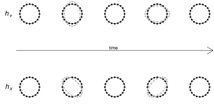
objects or two compact objects orbiting about each other. GWs can be described by oscillations in the fabric of space, causing space and everything in it to stretch and squeeze as the waves pass by. GWs do not travel through the space-time, rather the fabric of space-time itself is oscillating, i.e. GWs can be thought as “messengers”. In physics' symbols the gravitational wave measurements are denoted by “h”. We will talk more about what exactly “h” stands for, in next section. Also, since gravitational wave signals are measured with respect to time so the data are essentially a time series. In Figure 1, the effect of the GW passing through the plan of a ring of freely floating test masses is depicted. Each ring is situated in its own plan and all the plans are parallel and adjacent to each other. Each ring has an inner triangle whose vertices are situated at the three test masses of the rings. The superscripts of h, the “plus” and “cross” signs indicate the polarization of the GW. Polarization is a property of certain types of waves that describes the orientation of their oscillations. In describing GWs, it is useful to consider how they would act on a ring of free falling masses which in turn make it possible to estimate the sky-location of the source. A GW can travel in two polarizations known as plus polarization denoted by “h+” and cross polarization denoted by “h×”. In plus polarization,
the displacements of test masses of the rings occur in vertical as well as horizontal directions whereas the cross polarization occurs in the same manner but are rotated by 45° to plus polarization.
Figure 1 Illustration of the effect that a gravitational wave would have on a set of free falling test masses arranged in a circle. The wave's direction of travel here is orthogonal to the plane of the test masses. The wave's two orthogonal plus- (`+') and cross- (`×') components each cause an alternating `squeezing' and `stretching' into orthogonal directions, which are offset by 45o between plus- and cross-polarization. The overall effect is shown in the bottom panel, and it would have different appearances for different plus- and cross-amplitudes.
3.2 The Likely GW Sources
3.2.1 Galactic Compact Binaries: These types of binaries develop when two objects with very dense masses such as neutron stars (NSs) or white dwarfs (WDs), with roughly equal masses, orbit about each other. The compact objects move initially at an elliptical orbit about the common centre of mass. Over the course of time their individual orbits become increasingly circular as the two objects come closer and closer and at some point in time the two bodies appear to move around the centre of mass at the same circular orbit. This orbit decays with time like a spiral, as the two bodies come closer and closer to each other, which proceeds towards the common centre of the masses. Such spirals are called inspirals (in-spirals). As the two masses gradually inspiral, they emit gravitational radiation. These signals encode the luminosity distance to a binary, its sky location, and information about other physical parameters (Edlund et al. 2005, Nelemans 2009).
3.2.2 Mergers of Massive Black Hole Binaries: Similar to galactic binary systems are massive black hole binary systems in which both members are massive black holes with a
total mass in range 105M⊙-109M⊙. These sources will be detectable by LISA like detector (e.g. eLISA) at extremely large distances due to large masses involved. The GWs from these sources encode information about the masses and the spins of the two members. Once such sources are detected and the physical parameters are estimated, this information can be used to find out how these massive black holes are formed and what is the rate of their mergers, that is how often massive black holes encounter each other, which will put light on the evolution and structure of the large scale galactic dynamics (Berti et al. 2006, Berti 2006).
3.2.3 Intermediate and Extreme Mass Ratio Inspirals: It is predicted that most galaxies,
in their centres, host super massive black holes (105M⊙ -- 107M⊙) surrounded by a dense population of stellar objects such as NSs, WDs or small black holes and other normal stars. Due to multi-body interactions these stellar objects are often pushed into an orbit which passes too close to the central mass. The captured object then spirals in by orbital decay through the emission of gravitational radiation and eventually plunges into the central mass. Due to large differences between the two masses, such inspirals are called intermediate mass ratio inspirals (IMRIs) or extreme mass ratio inspirals (EMRIs) depending on the mass of central mass, and are one of the most exciting sources to be observed by Advanced LIGO and ET (Mandel et al.2008, Huerta and Gair 2011a, 2011b). The EMRI studies will help to understand the structure of the space-time around the SMBH using the physical parameters such as spin and mass, and the interactions between SMBH and the cluster of stellar masses around it (Barack and Cutler 2004).
GWs from these random and unresolved sources will form a very strong background noise which will be there in detector data stream and therefore will be of great importance for the precise detection of the other sources.
3.3 GW Detectors
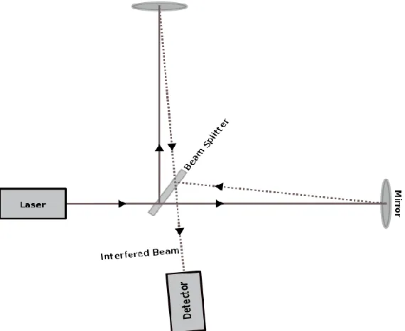
As shown above in Figure 1, the effect of GWs on free falling particles is that the distance between these particles changes as the wave passes by. The change in the distance, called strain amplitude and traditionally denoted by h, is used for measuring the effect of a passing GW directly. However, this change in the distance is extremely small and requires highly sensitive detectors. There are two types of detectors used for the detection of GWs. One is a resonant mass detector in which large masses are used and the deformation caused by GWs in them is measured (Fafone 2004, Aguiar 2011). The other type is a laser interferometer detector which actually works in a network of more than one detector located at sufficiently long distance from each other (Hough and Rowan 2005, Raab and the LIGO Scientific collaboration 2006). These detectors use the Michelson interferometry configuration, which works by splitting a light beam into two separate sub-beams that travel at different light paths along two arms of an L-shaped configuration. Mirrors at the ends of the arms reflect the beams back to the beam splitter, where they interfere upon being recombined. There are several GW detectors around the world that use this kind of interferometry. From the laser source, beams are sent to the ends of the arms where they are reflected by mirrors that are suspended by wires to work as approximately free-falling masses. When a GW passes through the plane of a detector the distance between the mirrors changes by a small amount, which is monitored by photo detectors that measure the phase change of the light. The distance between the masses changes by an amount ΔL, where L is the distance between the two masses, basically the arm-length of the triangle, resulting in a strain amplitude .
However, the gravitational wave effect is so week that a four km long arm ( ) can only give a ΔL ≤ 4 × 10-19m.
The currently operating ground based detectors can be divided into three generations according to their detection capabilities. The rst generation detectors are LIGO (Livingston, USA) and LIGO (Hanford, USA) ([Sigg 2004), GEO600 (Hannover, Germany) (Hild and the LIGO Scientific Collaboration 2006), VIRGO (Italy) (Acernese and the VIRGO Collaboration 2004), and TAMA300 (Japan) ([Takahashi and the TAMA Collaboration 2004) and a few other. These detectors are at most sensitive to gravitational radiation in the range 1104Hz. The response of ground based detectors to passing by gravitational waves is shown in the upper panel of Figure 3.
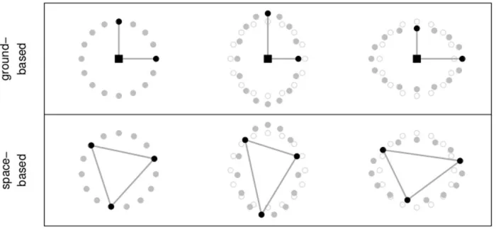
The LIGO and VIRGO are currently being upgraded to convert into second generation detectors by making some changes to their design and are called AdLIGO and AdVIRGO (Ad stands for advanced). The second generation detectors will be ten times more sensitive than their earlier versions. The third generation detectors include Laser Interferometer Space Antenna (LISA) (LISA website) and the Einstein Telescope (ET) (ET website). LISA is space-borne detector and was envisioned under a joint mission of NASA and ESA. The design of LISA allows to have very long arms and therefore is expected to be sensitive to low frequency gravitational radiation in the range 5×10⁻⁵— 10-1Hz. The basic detector consists of three freely flying spacecraft located at the vertices of an imaginary equilateral triangle configuration with L = 5×10⁹m long sides. Each spacecraft will carry two free-falling test masses and laser instruments that exchange laser beams with other two spacecraft to track the distances between the test masses within them to indicate the passage of a GW. The LISA triangle will move around the sun 20° (~ 5.2 × 10⁷ km) behind the Earth with its guiding centre (a point which is equidistant from the three vertices) at the Earth's orbit about the Sun (Vecchio2004, Cutler1998).
Due to budgetary problem NASA have withdrawn from this mission in October 2010 and now a scaled version of LISA, called eLISA is currently being investigated by ESA (eLISA website). The functionality and response of eLISA will approximately same as LISA, except that the arms of eLISA triangle will be a little shorter making it a little insensitive compared to LISA. The LISA/eLISA response to gravitational waves is shown in the bottom panel of Figure 3.
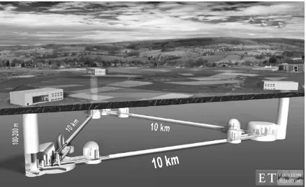
Figure 4: A design sketch of Einstein Telescope.
The more recently proposed Einstein Telescope is also being investigated in a collaboration of several European academic and space research organizations under the umbrella of ESA. A design study for ET is currently underway, which is exploring the design, cost, site selection, etc., plus the potential scientific impact of such an instrument, with a view to maximizing the scientific output within a reasonable budget. The design structures of ET and LISA are almost similar in the sense that both have three arms unlike the other L-shaped detectors. The detector is planned to be located 150m below the ground surface of the Earth with 10km arms as depicted in Figure 4. Different astrophysics and data analysis groups have started their work towards the future science goals of this detector. Mock data challenges have also been started to assess and develop the efficiency of GW templates and search algorithms for ET data analysis.
changes that occur due to the intrinsic nature of gravitational waves, the designed structure and position of the detector (plane) with respect to the origin of gravitational wave. These changes are adjusted using a mathematical formalism termed as detector response function. A detector response function is mathematically extensive so we leave its detailed explanations for our next article.
4. Bayesian Modeling 4.1 The likelihood function
The data, which is sampled at discrete time steps, can be represented by the following signal plus noise model,
where the deterministic component is the true signal model depending on parameters and is a zero-mean stationary time series with unknown spectral density (Röver et al. 2011).
Since the gravitational waves are periodic in nature and are recorded with respect to time therefore it is best to analyze them in frequency domain rather than in time domain. The reason is that in the frequency domain, we can see more of the salient features of signals that we cannot see otherwise. For example in the frequency domain, we may easily reshape a signal, enhance parts (frequencies) of it and suppress the other unwanted signals, isolate a primary signal from the influence of extraneous effects and much more. When the data are in (discrete) frequency domain for an unknown noise spectral density the likelihood function is defined as
̃ * ∑ ( ( ) ∑ ̃ ̃
)
+
where ⌊ ⌋ is the greatest integer less than or equal to , ̃ and ̃ are Fourier transformed observables and model signal, respectively, is the one-sided power spectral density and K is the normalizing constant. The noise spectrum, , is defined as,
| ̃ |
spectrum is assumed known then one can omit the constant term, log , from equation (4.2) to obtain
̃ * ∑ ̃ ̃
+
In the literature, equation (4.2) is known as Whittle's approximation to the Gaussian likelihood or simply Whittle likelihood (Whittle 1957). The Whittle likelihood assumes that the discrete Fourier transformed residuals are approximately independent complex normally distributed with mean zero and power spectrum . Another likelihood function in which the unknown noise spectral density, , is integrated out as a nuisance parameter was proposed in (Röver et al. 2011). The likelihood computation is commonly simplified by restricting the summation to a limited frequency range relevant to the signals of interest.
In the above likelihood functions the terms ̃ and plays the same role as μ and σ of a time domain Gaussian likelihood. In these terms, the index “j” in the above expressions may look confusing as it looks like ̃ and are also variables and for every data point there are a respective ̃ and values. However, by definition the two terms are still constants, it is actually the DFT which decompose a time domain signal into several frequency components. It is these frequency components that are represented by the subscript “j” and for every observed frequency in a DFTed data ( ̃ ) there is a corresponding frequency of parameter component ̃ ) as well as of a power spectrum component ( ) and the summation now runs over frequencies rather than time instants.
4.2 Why frequency domain approach?
4.3 Signal-to-Noise Ratio
A measure which is closely related to the likelihood function is the signal-to-noise ratio (SNR). It is an important measure in signal processing used for measuring the strength of the detected signal to the background noise. It is defined as:
√ ∫ ̃
(Christensen and Meyer 2001b) which for discretized frequencies becomes:
√ ∑ ̃
and for a particular frequency range the definition becomes:
√ ∑ ̃
(Cutler and Flanagan 1994) SNR is very useful as it measures the quality of the detected signal and hence of the parameters' estimates either on the fly or at the end of MCMC estimation.
4.4 The prior information
In the context of GWs the prior information refers to the information about (the range and the distribution of) the intrinsic/extrinsic and phase parameters of a source. Intrinsic parameters are those that represent the fundamental features of a source such as the mass, orbital frequency, eccentricity and the spin, whereas the extrinsic (such as distance and detector orientation) and phase (various phase angles) parameters are related to the projection of the information (through GWs) regarding the intrinsic features towards the outer space where a detector is to be located. In the light of astrophysical results and predictions the priors for all the parameters of sources can be easily established (see Arnaud et al. 2007 for more details). Furthermore, while doing the data analysis in a realistic manner, assuming that noise is unknown, one also needs to assume prior for the noise parameters which is also easy and can be done in several ways (see Röver 2007, Ali 2011 for example).
5. Examples
5.1 A simple sine-wave example
The first example is about recovering a simple sine-wave from a white noise background. A simple sine wave can be described by three parameters namely the amplitude ( ), the frequency ( ) and the phase ( ) parameter. The data model then takes the following form
where . Note that in these simplified examples the noise’s amplitude depends on the value of , i.e. and the detection and extraction of a target signal becomes harder if , that’s the noise’s amplitude is much larger than the target signal’s amplitude.
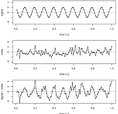
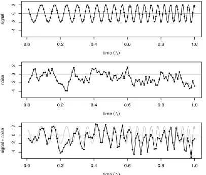
Let’s proceed with our example in which we take , and as our true signal parameters and . Data is generated for duration of a unit time (say one second) over discrete time points with an interval of . The signal, noise and signal plus noise (data) are plotted against time in Figure 5, which is self-explanatory. A Bayesian MCMC strategy was setup to extract the signal back from the data with prior information as , and . The results are given in Figure 6. We can see that the signal parameters are well spotted in just less than 2000 iterations and thus the signal can be easily reconstructed. Now let’s temper with noise’s amplitude by increasing the value of from 1.0 to 2.5 and see the consequences. We keep the signal parameters unaltered. The resulting MCMC search history is given in Figure [TracePlotsK3]. It is easy to conclude that for the same target signal if the noise amplitude was increased the MCMC will still find the true signal although it takes a bit longer. One can imagine the case when noise amplitude is several orders of magnitude larger than that of the target signal as it usually will be because of other sources of noise.
5.2 Several similar signals with different parameter values
According to astrophysical predictions, there will be millions of signals originating from millions of systems such as CBCs, SMBHBs, EMRIs and many others. Thus there will be hundreds of thousands signals from similar systems such as CBCs. Many of these systems can have almost the same characteristics values (e.g. having equivalent masses, distances, phases, orbital frequencies and other parameters), located at different places in the universe. For example there can be two almost equivalent CBCs situated at the almost same distances but different places in the sky.
Different parameters have different effects on the likelihood surface of the signal. In signal processing the most influencing parameters are those related to the amplitude of the signal. In the context of GWs, the amplitude mainly depends on the source’s mass, distance, and its location with respect to detector’s plane. The effect of mass and distance is easy to understand; it is directly proportional to the mass of the source and is inversely proportional to distance to the source. To explain the effect of location, we elaborate as to how a signal coming from different directions is received at a detector using the squeeze
Figure 5: A simple sine-wave signal, white noise, and signal plus noise (data). The dots denote the samples.
Figure 6: Trace plots of the three parameters and the posterior history for σ = 1.
and stretch phenomenon. If the signal is traveling perpendicular to the plane of detector (or test masses), it will be strong, and becomes weaker with the departure of its path of travel from perpendicular towards horizontal and it may not be even noticed if the path of travel is exactly horizontal to the plane of detector. It is actually related to detector response function and the sky location angles of the source. A detailed explanation of this phenomenon needs understanding the role and influence of relevant source and detector parameters, so we leave it for our next article. We have used a simple sine wave model, there were no mass, distance and sky location parameters given it were just simple parameter with some numerical value.
Now if we modify the dataset of the previous example by adding/injecting another (similar) signal with amplitude , while the values of other parameters remain the same. That is the only difference is the value of amplitude parameter. Thus there are now two signals in the data. In most of the MCMC runs this new signal will be picked up even if we start from the true amplitude ( ) of the first signal.
5.2.1 A chirping signal
Our second example is of a contaminated chirp signal. A chirp signal is one with instantaneously increasing frequency. In the language of gravitational wave processing community a binary is actually called a “chirping binary” rather than the more common word the “binary”. This example still does not depict a real binary, modeled by astrophysicists, generating a chirping signal because that modeled chirp is different in the sense that it also has increasing amplitude along with increasing frequency with time (this phenomenon will be explained in our next article). Here again, a time series of 100 points is generated by using the following equation with the deterministic component, , defined as below
̇
where the additional parameter ̇ is the frequency derivative (Röver et al. 2011). Here we use an AR(1) noise with uniform innovations (here ) within the interval
√ √ as the realistic astrophysical noise is understood to be colored (changing with time). The noise model takes the following form,
5.3 Some results on EMRI search in MLDC
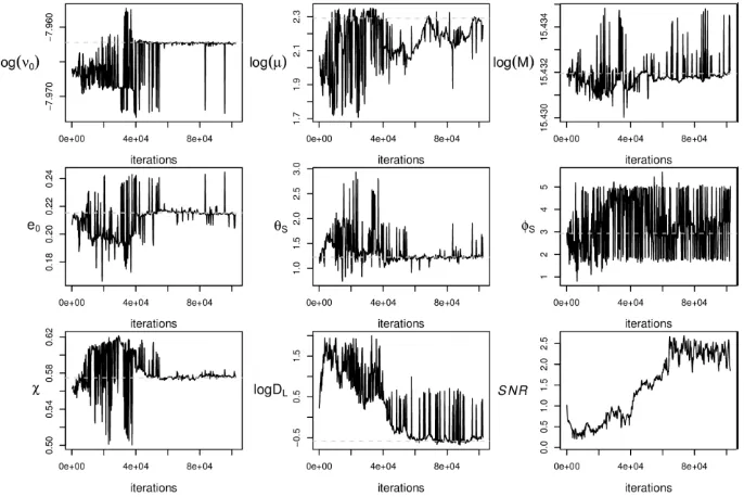
Here we present some results about EMRI detection and parameter estimation using LISA (now eLISA) data issued by Mock LISA Data Challenges (MLDC) task force during mission challenges. These results were part of A A's PhD thesis (Ali 2011) and also appeared in (Ali et al. 2012). For other types of signals such as MBH binaries the reader is referred to (Christensen and Meyer 1998, Christensen and Meyer 2001b, Cornish and Porter 2006, Röver et al. 2006, Röver et al. 2007). The details of EMRI signal template (Barack and Cutler 2004) and detector response, i.e. LISA response function (Cornish and Rubbo 2003) are mathematically extensive so we skip them for now. The intension is only to present some results that were obtained while participating in NASA MLDCs. Most of the mock data challenges consist of multiple stages called rounds. The complexity and purpose of these challenge data rises with each round. For example in the first round of MLDC was (a) the noise consisted only of LISA instrument noise (b) for each type of source separate data sets were generated, (c) there was only one signal of a particular source in a given data set and so on. In the first round the target signal is also kept a little brighter so that it can be easily detected. In the second round there were more complicated signals w.r.t parameter values. In the third round data set contained multiple signals from the same type of sources and the fourth round was called the “whole enchilada”, that’s there was only one data set that contained millions of signals from every possible source. EMRIs depend on 17 parameters of which 14 are important and were used/advised by MLDC task force for data simulation and likelihood computation. The large number of parameters and complicated nature of EMRI sources make their search and estimation a challenging task. The joint posterior surface of EMRI parameters contains multiple secondaries because a typical EMRI signal consists of several harmonics. The MCMC algorithm that we employed in these searches was a little advanced in the sense that it used parallel tempering MCMC (Geyer1991). Figure 10
Figure 8 A chirping signal, colored noise, and signal plus noise (data). The dots denote the samples.
shows detection results for the key parameters of a single EMRI source named as 1B.3.2 buried in LISA noise. One can easily see that the signal was well picked as the plot of SNR indicates.
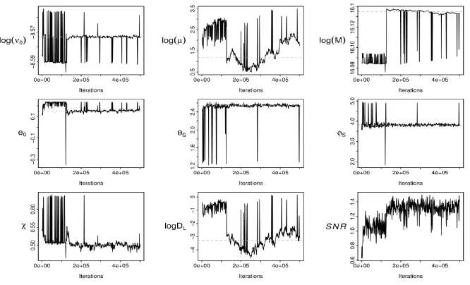
Figure 11 and 12 show the MCMC search and estimation results for blind data under MLDC round 4. The blind data set included 60+ million chirping Galactic binaries, 4 MBH binaries, 9 EMRIs, 15 cosmic-string bursts, an isotropic stochastic background, and instrument noise (Datasets website). These results were evaluated by MLDC taskforce (MLDC Taskforce website) and later presented in Amaldi 9 (2011) at Cardiff UK (Amaldi 9 website) and then listed on the website of TAPIR at Caltech (MLDC 4 results website). One member of the taskforce suggested that although the true signal was missed, but the sampler was still able a relevant secondary. That was a bigger success given the amount of noise ( millions other signals + instrument noise = overall noise).
Conclusions and outlook
We have demonstrated that the Bayesian MCMC approach for the detection and parameter estimation of signals that can be modeled using some mathematical formalism is quite simple and easy to apply. Although, the example signal models in this paper are very simple and apparently not very similar to realistic gravitational wave signals models but the GW signals are essentially same as these simple examples, except that their models will contain more details (number of parameters, observables, detector response adjustment, noises etc) about the nature of the source and data. We left the GW signals and their models for our next article where we will also discuss different GW sources, the nature of signals they generate and the waveform models in greater details. This paper also demonstrated as to how big a room there is for collaborations between astrophysics
and statistics communities. We wish to bring these two communities closer to each other to each other to work together in mutual scientific collaborations to participate in, and contribute towards, the international missions like LIGO, eLISA, ET and many others. Our group is currently associated with eLISA and ET data analysis and any offer of collaboration will be warmly welcome. In our next article, we will be discussing signals from different GW sources as predicted by astrophysics and relativity theories, such as CBC, SMBHB and EMRI, and discuss the Bayesian strategies used to detect these sources in a given detector data and estimate the various parameters associated with these sources.
Figure 11: MLDC 4 blind data: Trace plots of the 7 key EMRI parameters.
When the noise spectrum is assumed unknown, which is inevitable in realistic scenarios, then things become a bit more sophisticated, we will explain as to how to estimate noise as an unknown parameter in a Bayesian framework.
Acknowledgements
The work of Asad Ali was supported by Higher Education Commission (HEC) of Pakistan under SRGP fund with Ref No: PD-IPFP/HRD/HEC/2013/3029.
References
1. Amaldi 9, 2011 website http://www.amaldi9.org/.
2. Acernese, F. and the VIRGO Collaboration (2004). Status of VIRGO. Classical and Quantum Gravity, 21(5):S385.
3. Aguiar, O. D. (2011). Past, present and future of the resonant-mass gravitational wave detectors. Research in Astronomy and Astrophysics, 11(1):1.
4. Ali, A. (2011). Bayesian Inference on EMRI Signals in LISA Data. PhD thesis, The University of Auckland, New Zealand.
5. Ali, A., Christensen, N., Meyer, R., and R•over, C. (2012). Bayesian inference on EMRI signals using low frequency approximations. Classical and Quantum Gravity, 29(14):145014.
6. Allen, B. (1997). The stochastic gravity-wave background: sources and detection. In Relativistic gravitation and gravitational radiation: proceedings of the Les Houches School of Physics, pages 373-418.
7. Arnaud, K. A., Babak, S., Baker, J. G., Benacquista, M. J., Cornish, N. J., Cutler, C., Finn, L. S., Larson, S. L., Littenberg, T., Porter, E. K., Vallisneri, M., Vecchio, A., Vinet, J.-Y., and Force, T. M. L. D. C. T. (2007). An overview of the second round of the mock lisa data challenges. Classical and Quantum Gravity, 24(19):S551.
8. Barack, L. and Cutler, C. (2004). Lisa capture sources: Approximate waveforms, signal-to-noise ratios, and parameter estimation accuracy. Phys. Rev. D, 69(8):082005.
9. Berti, E. (2006). Lisa observations of massive black hole mergers: event rates and issues in waveform modelling. Classical and Quantum Gravity, 23(19):S785.
10. Berti, E., Cardoso, V., and Will, C. M. (2006). Gravitational-wave spectroscopy of massive black holes with the space interferometer lisa. Phys. Rev. D, 73(6):064030.
11. Bretthorst, L. G. (1988). Bayesian Spectrum Analysis and Parameter Estimation, Lecture Notes in Statistics. Number 48. Springer-Verlag, New York.
13. Christensen, N. (1992). Measuring the stochastic gravitational-radiation background with laser-interferometric antennas. Phys. Rev. D, 46(12):5250-5266.
14. Christensen, N. and Meyer, R. (1998). Markov chain Monte Carlo methods for Bayesian gravitational radiation data analysis. Phys. Rev. D, 58(8):082001. 2, 12
15. Christensen, N. and Meyer, R. (2001). Using markov chain Monte Carlo methods for estimating parameters with gravitational radiation data. Phys. Rev. D, 64(2):022001.
16. Cornish, N. J. and Crowder, J. (2005). LISA data analysis using MCMC methods. arXiv:gr-qc/0506059v1.
17. Cornish, N. J. and Porter, E. K. (2006). Mcmc exploration of supermassive black hole binary inspirals. Classical and Quantum Gravity, 23(19):S761.
18. Cornish, N. J. and Rubbo, L. J. (2003). Lisa response function. Phys. Rev. D, 67:022001.
19. Cutler, C. (1998). Angular resolution of the lisa gravitational wave detector. Phys. Rev. D, 57(12): 7089-7102.
20. Cutler, C. and Flanagan, E. E. (1994). Gravitational waves from merging compact binaries: How accurately can one extract the binary's parameters from the inspiral waveform? Phys. Rev. D, 49(6):2658-2697.
21. Edlund, J. A., Tinto, M., Krolak, A., and Nelemans, G. (2005). White-dwarf {white dwarf galactic background in the lisa data. Phys. Rev. D, 71(12):122003.
22. eLISA website. URL www.elisascience.org.
23. Fafone, V. (2004). Resonant-mass detectors: status and perspectives. Classical and Quantum Gravity, 21(5):S377.
24. Finn, S. L. and Cherno D. F. (1993). Observing binary inspiral in gravitational radiation: One interferometer. Phys. Rev. D, 47(6):2198-2219.
25. Gair, J. R., Porter, E. K., Babak, S., and Barack, L. (2008). A constrained Metropolis-Hastings search for emris in the mock lisa data challenge 1b. Classical and Quantum Gravity, 25(18):184030.
26. Gelman, A., Carlin, J. B., Stern, H. S., and Rubin, D. B. (2003). Bayesian Data analysis. Chapman and Hall/CRC, 2nd edition.
27. Geyer, C. J. (1991). Markov chain Monte Carlo maximum likelihood. In Computing Science and Statistics: Proc. 23rd Symp. Interface, pages 156{163.
28. Gregory, P. (2005). Bayesian Logical Data Analysis for the Physical Sciences. Cambridge University Press, New York, NY, USA.
29. Hastings, W. K. (1970). Monte carlo samping methods using markov chains and their applications. Biometrika, pages 97-109.
30. Hild, S. and the LIGO Scientific Collaboration (2006). The status of geo 600. Classical and Quantum Gravity, 23(19):S643.
32. Huerta, E. and Gair, J. R. (2011a). Intermediate-mass-ratio-inspirals in the Einstein Telescope. II. Parameter estimation errors. Phys.Rev., D83:044021.
33. Huerta, E. A. and Gair, J. R. (2011b). Intermediate-mass-ratio inspirals in the Einstein telescope. i. signal-to-noise ratio calculations. Phys. Rev. D, 83:044020.
34. Jaynes, E. T. (2003). Probability Theory: The Logic of Science (Vol II). Cambridge University Press.
35. Jeffreys, H. (1931). Scientific Inference. Cambridge University Press, 1st edn edition.
36. Jeffreys, H. (1939). Theory of Probability. The Clarendon Press, Oxford, 1st edn edition.
37. Loredo, T. J. (1990). From laplace to supernova sn 1987a: Bayesian inference in astrophysics. In Maximum-Entropy and Bayesian Methods, pages 81{142. Dartmouth, 1989, ed. P. Fougere. Dordrecht, The Netherlands: Kluwer Academic Publishers.
38. Loredo, T. J. (1992). The promise of bayesian inference for astrophysics. In Feigelson,E. D. and Babu, G. J., editors, Statistical challenges in modern astronomy, chapter 12, pages 275-297. Springer-Verlag, New York.
39. Mandel, I., Brown, D. A., Gair, J. R., and Miller, M. C. (2008). Rates and characteristics of intermediate mass ratio inspirals detectable by advanced ligo. The Astrophysical Journal, 681(2):1431.
40. Metropolis, N., Rosenbluth, A. W., Rosenbluth, M. N., Teller, A. H., and Teller, E. (1953). Equation of state calculations by fast computing machines. Journal of Chemical Physics, 21:1087-1092.
41. Nelemans, G. (2009). The galactic gravitational wave foreground. Classical and Quantum Gravity, 26(9):094030.
42. Porter, E. K. and Carre, J. A hamiltonian monte carlo method for Bayesian inference of supermassive black hole binaries. arXiv:1311.7539v1 [gr-qc].
43. Raab, F. J. and the Ligo Scientific collaboration (2006). The status of laser interferometer gravitational-wave detectors. Journal of Physics: Conference Series, 39(1):25.
44. Röver, C. (2007). Bayesian inference on astrophysical binary inspirals based on gravitational wave measurements. PhD thesis, The University of Auckland.
45. Röver, C., Meyer, R., and Christensen, N. (2006). Bayesian inference on compact binary inspiral gravitational radiation signals in interferometric data. Classical and Quantum Gravity, 23(15):4895.
46. Röver, C., Meyer, R., and Christensen, N. (2007). Coherent bayesian inference on compact binary inspirals using a network of interferometric gravitational wave detectors. Phys. Rev. D, 75(6):062004.
48. MLDC 4 Data sets.
http://astrogravs.gsfc.nasa.gov/docs/mldc/round4/datasets.html.
49. MLDC 4 Results website http://www.tapir.caltech.edu/~mldc/results4/index.html.
50. Sigg, D. (2004). Commissioning of ligo detectors. Classical and Quantum Gravity, 21(5):S409.
51. Stroeer, A., Gair, J., and Vecchio, A. (2006). Automatic bayesian inference for LISA data analysis strategies. AIP Conference Proceedings, 873(1):444{451.
52. Takahashi, R. and the TAMA Collaboration (2004). Status of TAMA300. Classical and Quantum Gravity, 21(5):S403.
53. Umst•atter, R., Christensen, N., Hendry, M., Meyer, R., Simha, V., Veitch, J., Vigeland, S., and Woan, G. (2005). Bayesian modeling of source confusion in lisa data. Phys. Rev. D, 72(2):022001.
54. Key Values, website,
http://pandora.aei.mpg.de/~steffeng/MLDC4/FullDataset1/svn1159/challenge4.0-training-key-frequency.xml.
55. Vecchio, A. (2004). Lisa observations of rapidly spinning massive black hole binary systems. Phys. Rev. D, 70(4):042001.
56. ET website, URL www.et-gw.eu.
57. LISA website, URL www.lisa.nasa.gov.
58. MLDC website, M. URL http://astrogravs.gsfc.nasa.gov/docs/mldc/who.html