THE APPLYING OF THE HARDWARE BASED RECONFIGURATION FOR AUTONOMOUS CONTROL SYSTEMS OF SPACE MOBILE ROBOTS

(1)

ISSN: 1992-8645 www.jatit.org E-ISSN: 1817-3195

13

EVALUATION OF COMPLEXITY OF THE LARGE-BLOCK

CLOUD COMPUTING USING ARITHMETIC WITH

ENHANCED ACCURACY

1_{VLADIMIR EFIMOVICH PODOLSKIY,}2_{SERGEY STEPANOVICH TOLSTYKH}

3

ANTON MIKHAILOVICH BABICHEV, 4SVETLANA GERMANOVNA TOLSTYKH

1

Tambov Regional Center of New Information Technologies 2,3,4

Tambov State Technical University Sovetskaya Str., 106, Tambov, 392000 Russia

E-mail:[email protected], [email protected], [email protected], 4

[email protected]

ABSTRACT

In the article, the methodological questions are considered of the complexity evaluation of large-block cloud computing with enhanced accuracy. The objective of our work is solving in the cloud of the mathematical simulation problems with special requirements for accuracy. In particular, we consider obtaining a precise and trustworthy solution for the problems with complex connections between sub-problems in the form of large blocks and the computation time considerably exceeding the time of information transmission between them. A methodology is proposed of the complexity evaluation for such problems used for creation of the optimal productivity computing systems, operating in a cloudy environment.

Keywords: Large-Block Parallel Computing, Cloud Computing, Precision Computation, Precise And Trustworthy Solution Of Problems, Floating Point Arithmetic With Enhanced Accuracy.

1. INTRODUCTION

The objective of the work is the cloud-oriented solving of a broad class of problems based on mathematical models with a complex topology. In addition, this class is characterized by a large volume of floating-point calculations with stricter requirements for the result’s reliability. Among such problems there are, for example, the problem of finding a partial system of combinations of the works on the water body recreation in an industrial region, the problem of designing a ventilation system in the enclosed bounded spaces with a complex configuration and many others. The problems of this kind require a responsible solution, because the obtained results may influence the volume of capital investments, life safety, or the rated quality of products. Similar problems were considered in the 80s in the works of G.M. Ostrovsky [1-3] devoted to decomposition of complex chemical-engineering schemes. In reality, the gain in computation time on the uniprocessor computers was achieved by finding an optimal iterated set (OIS) and reducing the

(2)

14 Currently, an opportunity has appeared to solve in the cloud the problems of global optimization not only in the deterministic case, but also in the conditions of uncertainty, which inevitably arise when the observability of the studied object is low. The amount of computation in such problems increases sharply in comparison with the deterministic setting, and a solution must be found in a multidimensional domain with the dimension greater than the dimension of the original deterministic problem. In the past, the solution of the optimization problems under uncertainty was usually limited to those rare cases when it was sufficient to solve simply the overall problem in terms of its localization to a single process or apparatus. Besides, in the conditions of strong nonlinearity of the constraints, it is practically impossible to obtain the solution of such problems by constructing the analytic convex hulls, and this increases the already high computational complexity. If, even in the conditions of analytically obtained convex hulls, we go to the level of the system of objects (for example, the shop floor), the need for high-performance parallelizing is obvious, as well as the fact that some elements of the computational system are large-block ones.

It should be noted that, when the dimension of the large-block problems of mathematical modeling increases, the understanding of the accuracy of the resulting solution is lost. Can one trust the obtained solution? If, for example, there are used in the calculations the multistage mathematical models of the kinetics of organic synthesis reactions, the reaction rates may vary by some orders of magnitude, and the system of differential equations becomes rigid. To such problems there are reduced the mathematical models of explosive processes, the processes of combustion and firing.

The practice of computing using the software packages of numerical methods gives reason to believe that even in solving the test problems associated with rigid systems, the precision of the floating point representation format of numbers with 16 decimal digits in the mantissa is not sufficient. It is necessary to engage the classes and/or functions for working with the arithmetic of enhanced accuracy. In this case, the time of calculation (particularly, involving standard mathematical functions such as exp(x)) increases dramatically. Even a low-dimensional problem which was before solved easily turns into a challenging computational problem.

It is not always possible to use the now traditional methods of parallelization developed for structurally simple problems (for example, for a number of problems in mathematical physics) with a very large number of similar elements (finite elements, finite differences). On the other hand, in the case of transition to a level, where an individual process vessel becomes an element of any significant system, there arises a tendency to consider a structurally simple element requiring the use of a powerful computing platform (cluster), so again there takes shape a large computing block, whereas the system as a whole becomes large-block.

The character of the parallel computing organization in the new conditions requires, above all, new theoretical justifications and methods of large-block parallelization in the cloud, taking into account the requirements of obtaining a precise and trustworthy solution and the possible presence of global iterative cycles in the calculation system. A motivation for the creation of a new theory is the need to evaluate the computational complexity as a minimization criterion: in the conditions of complicated calculation topologies it is important to correctly distribute the tasks with respect to resources, achieving a significant reduction in the total calculation time.

(3)

15 for example, a university computer network is used) [4].

In this article we use the terminology and notations used in the monograph [5]. The questions of the complexity theory were considered earlier by the authors in [6-9].

The studies are carried out in accordance with the Project No. 1346 from the register of state tasks for the higher education institutions and scientific organizations of the Russian Federation in the field of scientific research.

2. GENERAL THEORETICAL

STATEMENTS

We assume that the structure of the problem is known to us from the results of structural identification of the studied system S in accordance with the research goals (in reality, S is the initial system, for example, a shop floor for the acetylene manufacturing; a natural-industrial system of a region etc.); and this structure is a digraph G V , D , Γ , where V is the set of vertices, D is the set of arcs, Γ are the weight characteristics of the arcs. Next, n

V is the number of vertices, m D Γ is the number of arcs of the digraph of a structurally complex computational problem. It is required to find a digraph of the cloud computational system (CCS) for solving the original problem, so that the overall computational complexity becomes minimal:

∗_≡ ∗_, ∗_{, Γ}∗ _minΘ _,

where Θ is an estimate of the computational complexity of the digraph . The function characterizes the process of structural identification at the stage of the CCS synthesis.

Each of the arcs of the sought-for digraph identifies a calculation characterized by the following values:

1. Computational complexity Θ ; 2. The number of digits in the

mantissa in the realization of arithmetic operations;

3. The number ! of input variables that participate in the organization of the iterative process under the condition that this arc is cut.

We should note that in the simplest case (without aggregation of computations) the

parametricity γ_#, k 1, m is a functional of the form

γ γ Θ , & , ! .

We suggest

γ ! '(),*+, -*

, -* '

(.,*+/0 -*12k

0 -* ,

where

1. E_,,#4 1 is a parameter determined by experts, and is a measure of verification of the mathematical description of the simulated object with respect to the original system S ; for example, a phenomenological model usually has a higher measure of verification than a model constructed according to the "black box" principle and based on approximating the experimental data; into the parameter E_,,# one can include, for example, such indicators as the completeness of taking into account the factors and the correspondence to the studied phenomenon of the parameters of the mathematical model; thus, the parameter E_,,# expresses the preference for the mathematical description, and if it equals 1, the role of the computational complexity d_#of the arc in its resultant parametricity is minimal.

2. E_6,#4 1 is a parameter determining the increase of parametricity γ_# as the number of digits of the mantissa grows; it is natural to assume that, if for example, we want to compare the parametricity of two arcs, in one of which the number of digits equals 100, and in the other, 50, the latter is preferable for the iteration; on the other hand, a significant influence on the choice of the arc to be cut may have the amount of contours being broken: the bigger it is, the greater is the information load of this arc; we propose to evaluate this parameter as the contourness of the arc d_#;

(4)

16 computational complexity of this method is proportional to the cubed dimension of SLAE.

2.1. Basic notations and terms

We will assume that the digraph G is a result of structural identification of a cloud computational system (CCS) S, which is the object of study. The structure of the system is stationary, so the process of its identifying, the structuring Str S , is a mapping which associates to the system S a weighted digraph G

Str < : < → . (1)

The complexity estimate θ S is an integral quantitative characteristic of the overall computational load of the CCS, an indicator which facilitates ordering of various structures of CCS, proposed from outside, and choosing an option that has minimal complexity, other factors being equal [10].

The functioning of the system S is subject to the objectives of its existence, and this is reflected by an automorphism reflecting the purpose of calculations

@A < : < → <. (2)

The digraph G is the medium within which there are solved the problems T G T_C G , . . . , coordinated with Aim S .

Solving the problems from the tuple T G is carried out on the scale θ G after substituting the complexity estimates of the system S by the complexity estimates of the digraph

θ FG θ < . (3)

which means that “θ is a characteristic of θ < ” [5]. Such transition is correct only for the stationary and pseudo-stationary CCS, whose structure remains unchanged in time (or during some time, for the pseudo-stationary ones), or, in other words, for the systems, which are in the state of a classical block-scheme.

The digraph G is a tuple G V, D, Γ . The tuple G includes

− HI, @ 1. . J is the tuple of

vertices;

− FG HI→ HK , L

1. . A; @, N ∈ P1, JQ, @ R N is the tuple of arcs;

− Γ γ , L 1. . A; γ :=: is the

tuple of parametricities; the functor γ redefines γ and is a procedural model of the arc

parameterization process, γ :=: means " γ corresponds to ".

Further as the text goes, one may encounter the union of an arbitrary tuple with the empty tuple to the right from the concatenation sign: the operation does not change the content of the tuple, i.e.

∀A . . . , B . . . : B ⟸ A ∪ ∅ ⇒ |B| |A| .

However, if, as a result of concatenation, the empty element is to supplement the content of the tuple, we will use λ-functions in our notations:

B ⇐ A ∪ λ∅ ⇒ |B| \ |A| 1, where λ∅ ∅ is a

nameless tuple.

Hereinafter, in the graphic illustrations and some formulas, the vertices “v_^” may be denoted by aliases (auxiliary names) “i”.

The CCS digraph G has the following specific features:

1) parametricities are real scalars greater than one: γ 4 1. Thus, one plays the role of the reference value for parametricities. To the arc H_I→ H_K there is associated the

weight γ ∈ _`C,

L 1. . A, where _`C is the set of positive real numbers with the reference point 1. 2) let us confine ourselves to digraphs without

isolated vertices and multiple arcs, and this restriction corresponds to the condition ∃HI∈ : ∃N R @: HI→ HK∨ HK→ HI ∧

∃LC, Ld: e f.

(4)

(5)

17 Figure 1. Examples of digraphs for which condition (4)

does not hold:

digraph _C includes an isolated vertex, digraph _d

includes multiple arcs

2.2. Associative representations of the elements of the CCS digraph

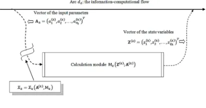
It is important to specify in advance what semantic associations arise in the representation of the CCS structure: what exactly is associated with arcs, and what, with the vertices? In our case, it is most convenient to assign the main computational load to the arcs, whereas the vertices act as servers, performing the distribution of information-computational flows. Figure 2 illustrates the semantic basis of the information-computational load attributed to an arc of the digraph. Note the following:

1) the arc has two possible states: the normal and the cut ones; in the latter the information-computational load includes not only the calculations, but also the functions of controlling the iterative cycle followed by a signal of completion/incompletion of iterations; 2) the information-computational load of the arc in the normal state is determined by the computational complexity of the calculation module M Z ; A , where Z is the vector of the state variables, resulting from the calculations, dimX j ; A vector of parameters that control the characteristics of computing in the calculation module, dimA .

3) the resultant information-computational

load of the arc in the condition of cut ' :=: k' may differ from the ordinary level dl :=:γm ; the more parameters are included into the vector A , i.e., the larger the number , the greater is the arc’s load.

4) selection of the arc for cutting and the subsequent organization of an iterative cycle is performed on the basis of total computational

complexity k ∘ γm , k' , where ∘ is the functional abstractor.

The essence of the information-computational flow is represented by a knowledge frame, it includes the procedural models M_# Z#; A# and γ# ∘ γm#, γ'# . The information component is represented in the flow by the vectors Z# and A#_{, whereas the computational one, by the above}

[image:5.612.318.524.317.425.2]

procedural models, and, if possible (if the arc is cut), by a procedural model of the arc cutting in the form of a predicate o_# o_# A#, M_# ∈ pfalse, truew. The value false corresponds to continuation of iterations, whereas true, to the end of cycle. In the case when all o_# true, k 1. . β∗ we take that the computational load in the system equals zero (here β∗ is the total number of the arcs being cut).

Figure 2. Computational Load Of An Arc Of The Digraph

2.3. Comparability of the CCS digraphs

The structural properties of a CCS digraph are expressed by the collection of two tuples: the tuple of vertices V and the tuple of arcs D. The parametric properties are expressed by the tuple Γ. The structural properties have priority in the graph ranking. It is necessary to introduce appropriate definitions.

Definition 1.

A weighted digraph G is comparable in structure with a non-weighted digraph G, this fact being denoted as G ⇄ G, if the weighted adjacency matrix of the weighted digraph G and the adjacency matrix of the non-weighted digraph G are equal up to the sign of the number

z{ |}J X ,_{|}J X ~ , •}€IK FG/γ:=:@ → N 1,

€IK FG/∃ @ → N ⇒ 1 ↬ 01, €IK G@ J €IKƒ ; @, N

(6)

18 where |}J X means that " is rendered concrete by X" [5], ↬ means "else".

Definition 2.

The weighted digraphs G_C and G_d are called identical in structure, this being denoted by GC~Gd, if

∃GC: GC⇄ GC, ∃Gd: Gd⇄ Gd, GC Gd

⇒ GC~Gd

(6)

The weighted digraphs may have the same structure and proportionally dependent parametricities.

Definition 3.

The digraphs G C and Gd, which are identical in structure and are similar in that the parametricities Gd can be obtained from the parametricities GC by multiplication by a positive coefficient, are called comparable, this being denoted by GC ⇌ Gd , if there holds the condition

C _{|}J X}_C _, d

|}J Xd ; ˆ€IKC

α €IKdŠ; @, N 1. . J, @

R N, α ‹ 0 … †F.

(7)

The notation of the form "y=con(x) " means "y is rendered concrete by x".

3. AXIOMATICS OF THE INTEGRAL

ESTIMATES OF THE CCS

COMPUTATIONAL COMPLEXITY (INITIAL STAGE)

To formalize the estimate θ G , we need a number of complexity axioms. They are the theoretical basis of derivation of the formulas for the quantitative evaluation of the CCS complexity.

Axiom 1 (on the estimates of complexity of comparable digraphs).

If G_C⇌ G_d and 1 Œ α Œ α, then they are comparable in complexity; moreover, if the complexity θ G_C is known, then the quantity θ Gd is proportional to θ G_C , namely

θ d • α θ C , • α : ∀α ‹∘: • ∘ Ž

• α Ž • α• , α• ‹ α. (8)

In formula (8), the function υ α acts as a constant of proportionality, while, in the formulation of the axiom, a restriction in the form of a double inequality is imposed on the value of α.

4. METHOD OF LEXICOGRAPHIC

NUMBERING OF THE STRONGLY CONNECTED DIGRAPHS

In accordance with the well-known axioms of complexity due to George Klir [11], the complexity of a system, consisting of a number of subsystems, is not less than the complexity of the entire system. At the same time, it is quite clear that a complexity estimate is constructive only when the George Klir’s axiom is fulfilled up to the "equality" sign for isolated subsystems. Therefore, formalization of complexity estimates should be agreed by the method of application to the indivisibility of the system into subsystems, i.e., in the development of estimates the system’s digraph should be strongly connected.

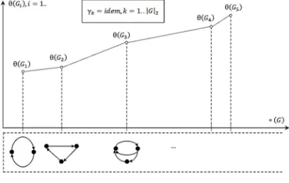
[image:6.612.317.521.455.584.2]

Hypothesis 1. If at our disposal we had a way of lexicographic numbering of strongly connected digraphs, then next there would arise a tendency to associate this numbering with the complexity estimates, i.e., to produce thus a digitization of the complexity scale (Figure 3).

Figure 3. Illustration To The Hypothesis About The Growth Of The Complexity Estimates Of Digraphs

Under Their Lexicographic Listing When The Parametricities Are Constant

To substitute the abstractor ∘ G to a specific function, we associate with the digraph G an invariant ‘ G , a unique integer

‘ : ∃ ′, ′ R ⇒ ‘ ‘ ′ ∧ ∀ ′ ⊂

: ‘ ‹‹ ‘ ‹ ′ .

(7)

19 ‘ G , and for any subgraph its invariant is always strictly less than the invariant of the digraph to which it belongs. In fact, ‘ G is an estimate of the structural complexity of digraph according to the number of its arcs. Besides the known axioms of complexity, this estimate takes into account a consistent statement: "If a digraph G contains more arcs in comparison with the digraph G”, it is more complex".

The idea of calculating the invariant ‘ G consists in accumulation of the bits starting from the low-order digits, according to the adjacency

matrix X, with the subsequent conversion of the bit strings into a non-negative integer.

(9)

where the operation "." is concatenation; "" is the empty string; "". €_IK is a bit string ("0" or "1", depending on the value €_IK 0 ∨ 1 ); the expression"0+bit_string" means that the "bit_string" is transformed into the corresponding positive integer; – — is the operation of taking the integer part of a number; ˜ is the complete digraph with the number of vertices coinciding with the number of vertices of the digraph .

Figure 4 shows an example illustrating the calculation of ‘ G .

(See in the appendix)

Figure 4. An example of a digraph invariant

5. STRUCTURAL DECOMPOSITION OF THE CCS DIGRAPH

In general, the CCS digraph may initially include strongly connected components (bicomponents) or, if they were not present initially, in the process of calculating θ G the digraph G is recursively simplified, and there appear bicomponents. Thus, it is necessary to formalize two radically different states of the CCS digraph:

1. digraph is strongly connected; 2. digraph is not strongly connected. In the first case, the reachability matrix

H š_{IK ›'›}, šIK {∃ @ →. . . → N ∨ @ N ⇒ 1, _{∃ @ →. . . → N ⇒ 0, @, N 1. . J} (10) is completely filled by ones; in the second, only partially.

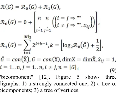
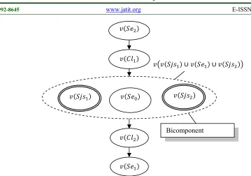
If reachability matrix has at least one zero element, then the digraph G of the system S contains at least two bicomponents corresponding to the strongly connected subsystems. In fact, a parallel is drawn between the concepts of a "strongly connected subsystem" and a

[image:7.612.319.521.117.279.2]

"bicomponent" [12]. Figure 5 shows three digraphs: 1) a strongly connected one; 2) a tree of bicomponents; 3) a tree of vertices.

Figure 5. Three variants of a digraph (bicomponents are in the ovals)

Figure 5 illustrates the need to consider three aspects of the formalization of θ G :

1) evaluating the complexity of trees of vertices;

2) evaluating the complexity of trees of bicomponents;

3) choosing the simplifying operations to bring a strongly connected digraph to the state of a tree.

6. AXIOMATICS OF INTEGRAL

ESTIMATES OF THE CCS

COMPUTATIONAL COMPLEXITY:

EVALUATION OF THE COMPLEXITY OF TREE-LIKE STRUCTURES

The structure of the tree-like CCS is described in the form of a tree of calculations [13]. A digraph G is called a tree (Remark 1), if it has no contours; and, to separate these digraphs into a separate class, we introduce for them a special notation Gœ.

To evaluate the complexity of trees, we formulate the following axioms:

[image:7.612.318.525.287.372.2]

(8)

20 A complexity estimate for the elementary tree with two vertices is no less than the weight of the arc that joins them.

˜ _C _{2, ˜} _d _{1 ⇒ θ ˜ 4 γ}_C, (11)

Axiom 2 (complexity estimate for the trees with comparable structures).

If the trees Gœ_C and Gœ_d are identical in their structure, Gœ_C~Gœ_d, and the total weight of arcs of the tree Gœ_C is greater than the total weight of arcs of the tree Gœ_d, a complexity estimate for the first tree cannot be less than a complexity estimate for the second one

ž γC, | ˜e|f

ŸC

‹ ž γd,

| ˜f|f

ŸC

⇒ θ ˜C 4 θ ˜d . (12)

Axiom 3 (on the relation between the complexity of a tree and a subtree).

The complexity of any subtree Gœ′ ⊂ Gœ is less than the complexity of the tree which contains it

˜′ ⊆ ˜ ⇒ θ ˜′ Œ θ ˜ . (13)

In accordance with the adopted axioms, two variants of formulas are proposed for estimating the complexity of trees, whereas each option is made agree with the set of axioms (11)-(13): Variant # 1 – evaluation of the tree complexity by the total weight of the arcs

θC _˜ _{ž γ}

| ˜|_f

ŸC

, (14)

Variant # 2 – evaluation of the tree complexity while taking into account the load of the paths

θd _˜ _{ž ž γ¡ ℙ}

,K |ℙ_*|

KŸC 0

ŸC

, (15)

where & is the total number of all possible paths from the vertices, belonging to the set of

exogenous vertices →£ of the tree ˜, to the vertices, belonging to the set of endogenous vertices ←¤ (see the illustration in Figure 6).

Figure 6. Illustration for the formula (15)

The selection of a criterion for the complexity evaluation of the CCS with a tree-like structure depends on the nature of calculations [14]:

1) A CCS < is a tree-like calculation module executed by independent computing devices. In such cases the estimate θC ˜ is suitable: it is an upper bound of computational complexity. On the other hand, this estimate can be used also in the case of distributed calculations with dependent computing devices, but not as a complexity estimate, but as an estimate of the overall computing capacity of CCS; this estimate can be used in designing the parallelization schemes: the smaller the computing capacity, the lower is the cost of the calculations themselves; there arises the problem of minimizing θC ˜ on the set of variants of the parallelization schemes.

2) The estimate θd ˜ can be applied to the cases where CCS is a collection of computing devices with a tree-like structure, whereas the main computational load is not on the arithmetic operations, but on the transmission of large volumes of information; a complexity estimate is proportional to the total loading of channels by the information flows during the stable period with a constant structure of calculations; the larger the average amount of information per a channel, the more loaded it is and the greater is the contribution of this channel to the overall complexity evaluation for the entire tree-like structure; for such cases, formula (15) is appropriate.

7. COMPLEXITY ESTIMATE FOR THE HIERARCHIC CCS

(9)

21 vertices. From the viewpoint of the graph theory, the structure of the hierarchic CCS is a tree of strongly connected subgraphs (SCS). To evaluate the complexity of the trees of SCSs (abbreviated as TSCS), it is necessary to convert TSCS into a tree of generalized vertices, a Hertz digraph, find the weight of the generalized arcs and apply to the obtained result the formulas for estimating the complexity of the trees of vertices [15-16].

Previously we adopted the concept that the complexity of calculations, concentrated in an arc, is associated with the weight of the arc, whereas the vertices are identified with the nodes of data distribution (data servers) (Remark 2). Extending this assumption to TSCS, it is quite logical to associate the complexity of an individual SCS with the weight of a generalized arc coming from the SCS. In the case when the SCS has several generalized arcs coming from it, the weight of each of them is reduced by as many times as there are generalized arcs coming from the generalized vertex.

On the conceptual level, to go from a tree of SCSs to a tree of vertices, we need a method of conversion of a tree of SCSs into a Hertz digraph, and this will require:

1) a method of unique concretization of SCS;

2) a method of evaluation of the SCS complexity;

3) a method of weighing the generalized arcs.

As a result, there will be formed a tree of generalized vertices, the complexity of which is evaluated according to the rules formulated earlier in the section 6.

7.1. Method of unique concretization of SCS

We need to construct a quasi-triangular form of the adjacency matrix X¦: X¦ con G , X¦:=:G, G ⇄ G, X¦:=:X, where X is the traditional non-weighted adjacency matrix of the initial digraph G. To this end, we turn to the method of constructing procedural models on the basis of operator equations.

A procedural model of construction a quasi-triangular form X¦ of the adjacency matrix X is verified by checking the following condition (which is illustrated in Figure 7):

①: λ β ≡ { ª@| «I\-I … †F, @ 1. . β : ® ∪_IŸC ¯

«I∪ -I °~ … †F ∧

∀βCŽ β: λ βC 0, -I:=:«I,-I KI, N 1. . ΥI, ²¦³:=:∪

IŸC ¯

«I∪ -I,

②: «Ie≺ «If≺. . . ≺ «I¶: ∀N ∈ P1, β \ 1Q: ∃· ‹ N: ∃L, ¸ He→∘ : He∈ «I¹º , (16)

where λ β is a λ -predicate, ª@| is the predicate equal to true, if digraph is strongly connected. The usage of a λ-predicate in this case if justified by that the first condition contains one and the same predicate twice, and it is the only one in this condition.

(See in the appendix) Figure 7. Illustration to the condition (16)

If a procedural model of constructing the matrix X¦ and the SCS G»_^, corresponding to this matrix together with the tuples of outgoing arcs -_^, i 1. . β, is written in the form of a conventional algorithm, then verification of the condition (16) is carried out as follows:

• there is formed a sufficiently representative (Remark 3) selection of initial digraphs

: ª@| ;

• to all paragraphs of this selection the procedure is applied of identifying the SCS, and the result is stored in an array of tuples;

• each of the elements of the resulting array is checked for the conditions ① and ②;

• if it appears that both two conditions are met for each element of the array, the conclusion is made about successful verification.

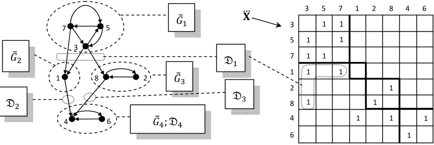
In Figure 8 there is given an example of construction of a tree of SCSs. In this example the digraph is split into three SCSs G con G»_C≺ G»d≺ G»¼ , whereas the corresponding tree has two

aggregation functors:

χC γC,#e..¾ ≡ χC γ 2 → 3 , γ 2 → 5 , γ 7 →

6 and χ_d γ_d,#_e..Â ≡ χ_d γ 3 → 1 , γ 5 → 4 , γ 6 → 1 , γ 6 → 4 .

Figure 8. Illustration to anti-lexicographic sorting of the

vector Ä

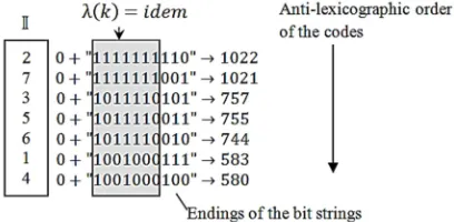
It should be noted that the SCS resulting from the anti-lexicographic sorting of the bit strings, the components of vector Ä, form a hierarchical structure.

A procedural model of searching SCS is a map Dec: G → G»^, -^, i 1. . β . We propose the

(10)

ISSN: 1992-8645 www.jatit.org E-ISSN: 1817-3195 22 F| ≜ Æ Ç Ç Ç Ç Ç Ç Ç

ÈÉ: 0 Ê Ä ÉË4 0 Ê Ä ÉËÌe, N 1. . J \ 1 ⇒ λ L 0 Ê

J .

KŸC

šK,

«_I Æ Ç Ç Ç Ç È Æ È

∀L ∈ ÉÍ..| «Î|: λ L @ FA;

· 1 Ê Ï 0:=:@ 1 ⋎ ž «_K

IÑC KŸC

Ò Ó Ô ⋏

-I Ö × ® H , H , , k ° :

∈ «I, ∉ «I

Ù ∘ ŸC Ó Ú Ú Ú Ú Ô

, @ 1. . β

Ó Ú Ú Ú Ú Ú Ú Ú Ô . (17)

Consider the expression (17). The result of calculations in the procedural model Dec is a permutation É/1. . n1 É_C, É_d, . . . , É_Û of the segment of natural numbers from 1 to n. If, following this permutation, we also simultaneously rearrange the rows and columns of the transposed adjacency matrix, we obtain a quasi-triangular form X¦, on the basis of which we find the SCS G»_^, along with a set of tuples of outgoing arcs -_^, i 1. . β. The condition of comparison of the elements, sorted in the anti-lexicographic order, is reflected by the inequality 0 Ê Ä_É_Ü4 0 Ê Ä_É_ÜÌe, j 1. . n \

1. The ending of the strings. Þ"" Êß

à Û

n \ i Ê 1 á

in the vector Ä serves for lexicographic numbering of vertices within the SCS, in accordance with the numbering of the vertices in the original digraph. Recall that the expression 0+ "bit_ string" is equal to an integer obtained from the direct binary code recorded in the bit string from left to right, starting from the most significant bit.

[image:10.612.93.297.562.662.2]

Figure 9 shows the result of sorting, it corresponds to the digraph in Figure 8. It is shown how the ending of the bit strings in the vector Ä helps building the numbers of vertices in the framework of SCS according to ascending of indices: for example, G»_C is characterized by the vertices v_d, v_â rather than v_â, v_d .

Figure 9. Illustration to the procedural model (17)

Note that, according to the above principles, to find SCS it is not necessary in the detection

process to find the contours of the digraph, one only needs to know the reachability matrix.

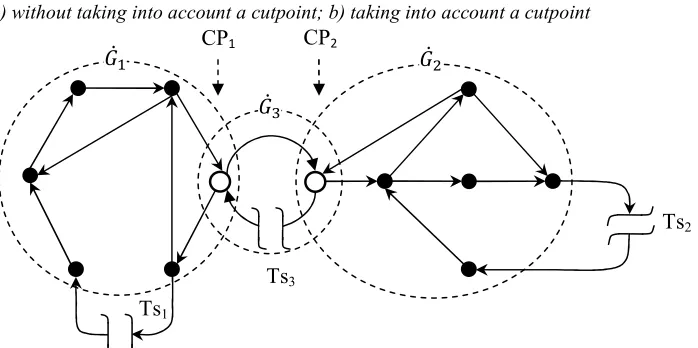
7.2. Method of searching SCS in the presence of cutpoints in the CCS graph

In some cases, evaluation of the computational load using the complexity estimates is made difficult by the petal topology of CCS, when the central place in the system is assigned to the cloud server with the protected data, or when a separate subsystem is formed by the cloud server, directly connected, at the same time, with several computing substations with a strong connected structure and, possibly, clusters. Figure 10 illustrates in a general form a grid-system aimed at solving a hypothetical problem with global iterations [17]. Consider the CCS digraph in Figure 11. It is shown without the cut arc corresponding to the global iteration cycle. The problem of structuring in which the cloud server, along with computing substations, is combined into a single bicomponent, is that all three elements are considered as a whole; the iteration cycles may contain undesirable association of the cloud server with the vertices belonging to computing substations, as shown in Figure 12. The variant b) is different in that, as a result of decomposition, there are found two contour SCSs instead of one component as in the variant a), these are Gã_C and G»d. The working of the computing substations

corresponding to these SCSs, is now controlled by two iterative cycles Ts1 and Ts2, and, at that, the cutpoint CP does not lose its significance as the coordinator of computations. In this case (Remark 4) the complexity estimate is equal to the total complexity θ Gã_C∪ Gã_d θ Gã_C Ê θ Gã_d .

In some cases, the cloud server can be regarded as an independent subsystem as shown in Figure 13, then the number of cutpoints increases. If the cloud server is connected to two substations, it is natural to assume that there are exactly two cutpoints in the Gã_¼ subsystem, i.e., their number is equal to the number of substations associated with the server.

(11)

23 communication of the general geographic scope [18-19].

Note also that, as a cloud server, there can be, for example, the branch server. With regard to the problems of organization of high-performance cloud computing, such situations are possible, for example, when solving systems of equations of large dimension, divided into two (or more) blocks with one (or more) equation on the separation boundary (the equation of conjugation [20]). In such cases, one can find a permutation of the rows and columns of the adjacency matrix, applying which this matrix acquires a pseudo-quasi-diagonal form, as shown in Figure 14.

Generally speaking, bicomponents and the contour subgraphs may be considered strongly connected subgraphs of different types, and, on formal grounds, in a digraph either types can exist simultaneously. However, a differentiated approach to the enumeration of subgraphs (with their subdivision into types) significantly complicates the further formalization. It is reasonable to equate bicomponents, in which there are no cutpoints, with the contour subgraphs if we use a bouquet model of decomposition. The choice of the specific procedural model of the digraph decomposition into SCSs depends on the specific situation in which the complexity is evaluated by gradual simplification of the system under study with the further composition of the estimates of primitive structures, going up from the lower level of decomposition. With respect to cloud computing, one of the factors in favor of the method of contour subgraphs is the original structure of connecting of cloud servers. For example, if there are connections of the "star" type in the scheme and the problem is set of evaluating the stability of working of the cloud system, then the contour subgraphs are preferred over bicomponents.

Figure 10. Example of a grid system with global iterations and a cloud server

Figure 11. Structuring of a grid system: the case of one bicomponent

Figure 12. Variants for decomposition of the CCS digraph in Figure 11:

a) without taking into account a cutpoint; b) taking into account a cutpoint

Figure 13. The variant of structuring, when the cloud server is represented as a contour SCS

Figure 14. General form of the adjacency matrix for a system of equations of large dimension with the equation

of conjugation of blocks

8. THE METHOD OF

STRUCTURAL-PARAMETRIC MINIMIZATION OF

THE CCS DIGRAPH

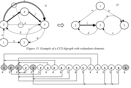
A CCS digraph may contain the elements that contribute to an increase in computation time of the complexity estimation, which adversely affects the application of these estimates in the online regime. Among these elements, hindering the analysis of complexity, there are the branches of calculations performed serially and hidden parallel branches of calculations. In Figure 15 there are shown: an example of the digraph (G), including redundant elements, and the result of structural-parametric minimization (SPM), the digraph G’.

Figure 15. Example of a CCS digraph with redundant elements

Transitive computational flow 2 → 4 → 5 (the arcs are highlighted by thick lines) is replaced by the generalized arc 2 ⇒ 5, its parametricity is shown in Figure 15 in the form of a question mark: it is required to determine how it will be evaluated. Through the generalized arc (such arcs are marked by double lines) 2 ⇒ 5 there goes computational flow, which is performed parallel to the computational flow in the initial arc 2→5 of the CCS digraph (it is marked by circles and by dotted line connecting them): these arcs have the same initial and end vertices. The parametricity of the generalized arc of the digraph G’ is also shown in

the form of a question mark.

Evaluation of the complexity of parallel computational flows should take into account the character of their carrying out: if these flows are processed in parallel, then the complexity evaluation must be coordinated with the critical line, whose complexity is maximum.

(12)

(13)

25 analysis of the previously analyzed structures, there are used the accumulated knowledge with the ready answers. The first in the list of the tested and ready to be included into the database knowledge there should be strongly connected digraphs of small dimension, consisted of 2 and 3 vertices. For them, we need to derive the complexity estimation formulas.

The criterion ‘ G (formula (9)) allows ordering the list of strongly connected digraphs, which are representation of the simplest topology of iterative and cyclic calculations. We need to remove from this list isomorphic digraphs, and, for the remaining digraphs, to find the estimation formulas for the complexity θ (G) in the form of absolute predicates.

It should be noted that in the criterion ‘ G the weight of the arcs is not used and ∀G: G G ⇒ G ⇐ G\Γ. Beyond the issues of indexing of the list elements, in this section we will use the restored G ⇐ G ∪ Γ.

Consider the codes of all possible strongly connected digraphs with three vertices, ranking them in the order of increasing of the criterion ‘ G : 23, 25, 27, 29, 31, 38, 39, 45, 46, 47, 54, 55, 57, 58, 59, 61, 62, 63. Due to its uniqueness, the criterion ‘ G is taken as the basis of constructing the isomorphism diagrams for the class of strongly connected digraphs with the given vertex dimension |G|_C. The arrows in these diagrams go from right to left, coming to the codes of the basic digraphs. Figure 17 shows the results of studying the isomorphism of the above-mentioned list of digraphs according to the criterion ‘ G , in the form of a diagram of isomorphisms. A failure with respect to the arc dimension |G|_d is observed immediately, starting with the code 23: there corresponds to it a digraph with 4 arcs, whereas to the code 25 there corresponds a digraph with three arcs. There is clearly a violation of the principle of assigning the invariants (9). In Figure 17, the basic codes are marked in gray, i.e. the corresponding isomorphic digraphs have the code ‘ G , the value of which exceeds the basic code.

Figure 17. The codes ‘ of digraphs with three

vertices and the number of arcs (below)

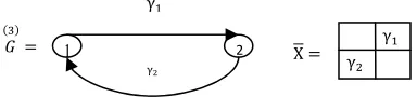
10. COMPLEXITY OF A DIPOLE

A dipole is a strongly connected digraph; let us

adopt for it the notation of the form G

¼

, where the

superscript “3” is the value of the invariant

‘ z G¼„. There are two vertices and two arcs in the dipole:

¼

, , Γ , HC, Hd , C, d,

C HC→ Hd, d Hd→ HC, Γ γC:=: _C, γ_d:=: _d.

(18)

The dipole G

¼

[image:13.612.321.513.296.341.2]

is shown in Figure 18. It is a mathematical description of the structure of the simplest CCS. The dipole vertices correspond to the blocks of the information distribution (servers), whereas the arc, to the computing resources (computers, clusters, cloud platforms) [21].

Figure 18. A dipole and its weighted adjacency matrix

Evaluation of the complexity of systems is produced by a series of simplifications implemented in the same way. In the cognitive subtext, a series of simplifications can be represented as a tree of recursion when calculating the complexity estimates, as it is demonstrated in Figure 19.

The structure of the initial state of CCS is represented by a strongly connected digraph

G R G¼, bic G true. It is required to estimate the computational complexity of CCS. For this purpose, the initial digraph undergoes gradual decomposition. The initial state of the digraph is assumed to be the zero stage. With regard to CCS, it is the dipole that is the final structure in the tree of recursive calculation of the complexity estimate.

In the process of evaluating the complexity of large-block calculations with global iterations it is a dipole that is a crucially important CCS. Finding a way to transform a dipole into the disconnected state, and simultaneously making the complexity evaluation, one can evaluate the complexity of the entire CCS. At that, in addition to the dipole one must be able to evaluate the complexity of the trees of calculations (see sect. 6).

Figure 19. An example of tree recursion: is the CCS

digraph in its original state; Β 3_{is the number of}

γC

γd

X _γ γC

d

1 2

(14)

26

levels of hierarchy; β_I, @ 0. . Β is the width of the levels

in the tree of recursion

Returning to Figure 18, it is easy to notice the presence of two alternatives for disconnecting a dipole: either a break of the arc (1→2), or a break of the arc (2→1). In CCS a break of any arc is connected with the need to iterate with respect to one or more variables, transmitted as a result of the information distribution at the vertices for the subsequent calculation in the arcs of digraph. To resolve the alternative, it is necessary to take into account that the arcs are a topological representation of the computational process, and the choice of the arc, along which the iteration is to be performed, is determined by the complexity of arcs and their articulation in the CCS digraph. We should at once make a reservation that, before calculating the overall evaluation of the complexity of the entire CCS, the parametricities of all arcs of the digraph, without exception, should to be known beforehand.

Procedurally, a computing dipole can be conveniently presented as a CCS with alternative choice of the iteration order: either the cut of the arc d_C is a procedural realization of sect. 2, or, conversely, the arc d_d acts as such. Figure 20 shows a graphical interpretation of the procedural model of a dipole as an iterative CCS. A dipole has "input" and "output": at the input there is performed taking off the information, the vertex v_C is marked by the sign "-", whereas the vertex v_d, at the output by the sign "+", respectively: it is the returning of information. In this case, the dipole can be considered as non-automorphic digraph.

¼

~ ′¼,¼ pHC, Hdw, p C 1 → 2 , d 2 → 1 w ,

′

¼

pHd, HCw, p C 2 → 1 , d 1 → 2 w .

(19)

In the procedural block "a" there acts the mapping w_C, producing transformation of the original information, the vector of tuples x into a subvector x_Cd ⊏ x ; there takes place the refinement of the composition of the initial approximation with respect to the reverse calculation flow coming from the "+" -vertex of the dipole to its "-" -vertex. The switch Sw0 changes the course of setting the initial approximation and, thus, the order of iteration cycles. In the "on" position, the initial information is sent to the procedural block "a", whereas in the "off" position, the initial information, the vector of tuples x , is sent to the vertex of the dipole with the indication "-", into the procedural block "b",

where the selection of information for the vertex 2 is carried out by the mapping w_d.

Figure 20. Dipole as a procedural model of iterative CCS

The main computational load falls on the blocks "c" and "d". There act the maps ϕ_C and ϕ_d, the calculations are carried out in the direction from the vertex labeled by "-" to the vertex labeled "+" (ϕ_C) and, vice versa (ϕ_d). In the comparators "e" and "f", there is performed the calculation of the predicates UC,d • and, if the predicate is true, then the calculations are finished, "Exit". Otherwise, the information, previously obtained from the procedural blocks "b" and "c", is passed to the vertices of the dipole for further iterations. On the way from the vertex to the procedural block there are the switches Sw1 and Sw2 (the down arrow means "the way is closed", the up one, on the contrary, means "the way is open"). They control the operation of the dipole; in any case, there operate either one of the comparators or both. It is necessary to determine how exactly the comparators are set, there depends on it the overall computational complexity of the dipole: it should be minimal; an estimate of the total complexity of the CCS digraph is built on this.

An estimate of the dipole complexity includes two quantities:

1. Complexity of the simplification procedure θ_ì, as a result of which the dipole becomes a tree (the index "s" stands for "simplification");

2. Complexity of the arc θ_í, obtained as result of simplification (the index «r» stands for "residual", i.e. θ_í is the residual complexity).

Let us formulate the axiomatics. Taking into account that in the working of dipole there are possible two variants of turning on the comparators, then the axioms are also two.

Axiom 5 (complexity of the dipole with one comparator).

(15)

27

θ z¼„ 4 θîí≡ θîÊ θí. (20)

Axiom 6 (complexity of the dipole with two comparators).

In the general case, the estimate of the dipole complexity is calculated as a minimum of two estimates: the complexity estimate for iterations, resulting from the cut of the arc 1→2 and a similar estimate for the arc 2→1

θ z¼„ minpγC 1 Ê γd , γd 1 Ê γC w. (21)

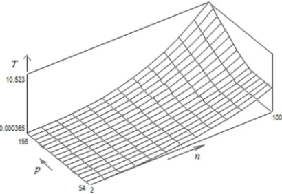
[image:15.612.92.297.420.561.2]

It should be noted that in the future the formula (21) will have to be concretized for the catalog of typical blocks associated with the computational methods. For the non-typical blocks it is necessary to obtain the experimental characteristics: the parametricities γ_C and γ_d as the functions of the calculation accuracy and the characteristics of the dimension of the problems being solved. In the Figure 21 there is presented the experimental dependence of the calculation time for the Gauss method of solving the systems of linear algebraic equations as a function of the dimension n of the system and the number p of digits of the mantissa p.

Figure 21. Dependence of the calculation time for the system of linear algebraic equations (sec.) on the dimension of the system and the size of the mantissa

To approximate the experimental dependence shown in Figure 21, we used the dependence

T n, p αn¼_pd_{Ê βn}¼_pÊγnd_pd_{Ê δn}d_p _.

Particularly, for the Gauss method we obtained the following values: 10-10×(α 1.88, β 59.1, γ 10.4, δ 184 . Similar studies were carried out for a number of methods for solving linear algebraic systems, the approximation coefficients were found. The obtained data led to the conclusion about the applicability of formula (21):

the maximum deviation in the case, when in the dipole arcs there participated the solution of linear algebraic systems, did not exceed 5% of the relative error.

11. PROCEDURAL MODEL FOR

EVALUATING THE

COMPUTATIONAL COMPLEXITY OF CCS

One of the outcome of the development of a methodology for assessing the computational complexity of CCS is a procedural model, which takes into account all aspects of the developed theory.

1. Input (recursive adapter): digraph , , Γ .

2. Is the digraph strongly connected? ª@| 1? If "yes", then go to item 12.

3. Structural decomposition: subdivide into SCS_I, @ 1. . β.

4. θ 0.

5. Cycle over SCS_I, @ 1. . β.

6. Input (recursive adapter): digraph G

= SCSi.

7. θ θ Ê θ.

8. End of the cycle over i.

9. ô ô .

10. Output: θ.

11. Up to isomorphism, is the digraph G

present in the knowledge base of complexity estimates (the knowledge base is indexed by invariants of strongly connected digraphs)? If "Yes", then make an inquiry into the knowledge base, obtain an estimate

θ ≡ θ and exit the recursive

adapter with the value θ.

12. Carry out SPM of the digraph mın

ö÷÷÷÷÷÷ø .

13. Construction of the matrix of contours Cú .

14. ô ûü ý_ (the largest of all

possible real numbers in the С++ language).

15. Cycle over the arcs of the matrix of contours, @ 1. . A.

16. Cut of the arc ′ \p _Iw.

17. Input (recursive adapter): G = digraph ′

(16)

28 19. θ Ž θ ? Is the estimate decreasing?

If "NO", then exit the cycle over i. 20. Store the estimate θ θ.

21. End of cycle over i. 22. Exit with the value θ θ .

12. CONCLUSION

A theoretical basis is developed for evaluating the complexity of large-block cloud computing, using the arithmetic with enhanced accuracy, which includes the methods and procedural models intended for designing CCSs. Currently, the work is underway towards the further elaboration of the complexity estimates for real-world computing dipoles. The computational experiments are carried out on the use of the arithmetic with enhanced accuracy in various numerical methods with the further approximation of the obtained results of testing. It is planned to obtain specific expressions for the parametricity functionals of the arcs of the CCS digraph in solving a number of large-block problems of mathematical modeling.

REFERENCES

[1]. Ostrovsky, G.M., 1975. Optimization of Complex Chemical-Technological Schemes. Moscow: Khimiya.

[2]. Ostrovsky, G.M., 1980. Decomposition of Complex Chemical-Technological Schemes.

Moscow: Khimiya, 1980.

[3]. Hansel, K., Yu.M. Volin and G.M. Ostrovsky, 1980. Methods of Structural Analysis in the Problems of Studying Chemical-Technological Schemes. Vol. 4 (89). Moscow: NIITEKHIM.

[4]. Zykov, A.A., 2004. Fundamentals of the Graph Theory. 3rd Ed. Moscow: Vuzovskaya Kniga, pp: 10.

[5]. Podolsky, V.E. and S.S. Tolstykh, 2006. Improving the Efficiency of Regional Educational Computer Networks Using the Elements of Structural Analysis and

Complexity Theory. Moscow:

Mashinostroenie.

[6]. Tikhonov, A.N., S.V. Mishchenko, V.E. Podolsky and S.S. Tolstykh, 2004. Features of Mathematical Modeling of Modern Computer Networks in Education (Vol. 1). St. Petersburg, pp: 78-79.

[7]. Tolstykh, S.S. et al, 2009. Constructing of the Optimal Block-Concurrent Calculation Modules in a Distributed Computing Environment. In New Information Technology and Quality Management: Proceedings of the International Symposium, Turkey, pp: 160-162. [8]. Fedorov, R.V., Yu.V. Osetrov and S.S. Tolstykh, 2009. Designing the Architecture of a Scientific Information System to Support the Study of Structural Complexity. In V.P. Gergel (Ed.), Microsoft Technologies in the Theory and Practice of Programming. Conference Materials, Nizhny Novgorod: Publishing House of the Nizhny Novgorod State University. [9]. Mainika, E., 1981. Optimization Algorithms on

Networks and Graphs. Moscow: Mir.

[10]. Lipaev, V.V., 2001. Providing the Software Quality. Methods and Standards. Moscow: SINTEG.

[11]. Klir, G., 1990. Systemology. Automation of the Solutions of System Problems. Moscow: Radio i Svyaz.

[12]. Casti, J.L., 1982. Large Systems. Connectivity, Complexity and Catastrophe. Moscow: Mir.

[13]. Savage, J.E., 1998. Computational Complexity. Moscow: Factorial.

[14]. Razborov, A.A. About Computational Complexity. Mathematical Education, 3: 127-141.

[15]. Kuzyurin, N.N. and S.A. Fomin, 2007. Efficient Algorithms and Computational Complexity. Moscow: MIPT.

[16]. Lazdin, A.V. and O.F. Nemolochnov. Complexity Estimate for the Graph of a Functional Program. Scientific and Technical Bulletin of SPbGITMO (TU), 6: 112-117. [17]. Voevodin, V.V. and Vl.V. Voevodin, 2002.

Parallel Computing. St. Petersburg: BHV-Petersburg.

[18]. Tarasov, A.G., 2009. Expandable Monitoring System for a Computing Cluster. Computational Methods and Programming, 10: 147-158.

(17)

29 2006 (Vol. 1), St. Petersburg: St. Petersburg State University, pp: 253-258.

[20]. Nicolis, G. and I. Prigogine, 1990. Exploring Complexity. Moscow: Mir.

(18)

30 Remarks

1. In this case, a specification is appropriate: a tree of vertices.

2. An alternative is the load on the vertices in the form of a vertex potential. In our opinion, such an approach may greatly complicate the evaluation of complexity, especially when the digraph is strongly connected. Under such approach, any calculations associated with the estimates of complexity presuppose solving the Kirchhoff system of equations.

3. The issues of completeness of the digraph selection are not considered here, it is a separate research topic.

4. In order not to confuse the contour SCSs with bicomponents, we will use as superscript not "~", but the sign "."

[image:18.612.96.477.370.482.2]

APPENDIX

Figure 4. An example of a digraph invariant

Figure 7. Illustration to the condition (16)

«

_C

«

_d

«

_¼

«

;-∅

-

C

-

d

-

¼

1 2

3

4

5

6 7

8

3 5 7 1 2 8 4 6

3

5

7

1

2

8

4

6 1

1 1 1

1

1 1 1

1 1

²¦

1 2

3

X

1

1 1

‘ =1111012 = 61

‘ ˜ 63, L –log_d63 Ê 1/2— 6 ⇒ ‘_C 2 Ê 2âÊ 2 Ê 2 Ê 2C 1984

[image:18.612.92.522.550.694.2]

(19)

(20)

[image:20.612.122.481.68.320.2]

32

Figure 11. Structuring of a grid system: the case of one bicomponent

H <NGC

H ·C

H ·d

H <F H <NGd

H H <NGC ∪ H <FC ∪ H <NGd

H <FC

H <Fd

(21)

[image:21.612.92.526.61.532.2]

33

Figure 12. Variants for decomposition of the CCS digraph in Figure 11: a) without taking into account a cutpoint; b) taking into account a cutpoint

Figure 13. The variant of structuring, when the cloud server is represented as a contour SCS

Ts1

Ts2

ã

C

ã

d

CP1

CP2

ã

¼

Ts3

PTs0 «_C≔: H H <NG_C ∪ H <F_C ∪ H <NG_d

ô «C ?

a)

b)

«_C

Ts0 CP

Ts1

Ts2

ã

[image:21.612.161.510.537.711.2]

(22)

[image:22.612.99.522.68.317.2]

34

[image:22.612.244.515.151.315.2]

Figure 14. General form of the adjacency matrix for a system of equations of large dimension with the equation of conjugation of blocks

Figure 15. Example of a CCS digraph with redundant elements

Figure 17. The codes ‘ of digraphs with three vertices and the number of arcs (below)

2 2 2 2 3 3 3 4 4 4 5 5 5 5 5 6 6 6

3 3

4 4 4 5 4 4 4 5 4 5 4 4 5 5 5 6

2 5

4

c f

?

d

3 1

a

b g

e

h

1

2 ? 5 3

a _b

d e

h

G’

G

Pseudo-quasi-diagonal

1st block of

equations

2st block of equations

– zeros

– zeros and ones

[image:22.612.93.520.363.650.2]

(23)

[image:23.612.102.524.57.478.2]

35

Figure 19. An example of tree recursion: is the CCS digraph in its original state; Β 3_{is the number of} levels of hierarchy; β_I, @ 0. . Β is the width of the levels in the tree of recursion

¼

C,C C,d

¼

C, e

¼

d,C d,d

¼

d, f

¼ ,C

¼ ,¯

Zero level of recursion,

β 1

D

ir

ec

ti

o

n

o

f

d

ec

o

m

p

o

si

ti

o

n

βC 3

βd 3

The lower level of recursion, the level of dipoles,

β 2, Β 3

(24)

[image:24.612.99.518.71.396.2]

36

Figure 20. Dipole as a procedural model of iterative CCS

No

Cd →_e C

1

C _→

e C

C _üC _• _{… †F?}

Input:

CC →_f d

üd _•

… †F?

d _→

f C

d No Sw

Output: _C Sw2

→

e C

d

– Dipole ₊

а

c

d 2 e

f →

f C

C Sw