Laboratory Test System Design for Star Sensor
Performance Evaluation
Jun Yang, Bin Liang, Tao Zhang, Jingyan Song and Liangliang Song
Department of Automation, Tsinghua University, Beijing, ChinaEmail: [email protected]
{bliang, taozhang, jysong}@mail.tsinghua.edu.cn
[email protected]
Abstract—A novel laboratory test system is designed to evaluate the performance of star sensors. Two evaluation methods are presented, the star images simulation test and the zenith observation experiments method. In star image simulation, the nebula and moon lights enter into the CCD field of view (FOV) is considered. A new algorithm for fast access star catalog is also designed to enhance the speed of star image simulation. Zenith observation provides a new method to test accuracy of star sensor without telescope. The results demonstrate that the test system is effectively to evaluate the star pattern recognition rates and relatively accuracy performance of star sensors.
Index Terms—Star sensor, Star image simulation, Zenith observation, Catalog, FOV
I. INTRODUCTION
With the booming of the space exploring, accuracy attitude determination and autonomous navigation becomes the crucial requirements of the spacecrafts. Star sensors can meet both of requirements above and its accuracy is much higher than other sensors, such as sun sensor, gyroscope, magnetometer, horizon sensor and etc [1]. Star sensors have been widely used to provide high accuracy attitude for the spacecrafts missions. With the extending complication of missions, low-mass, low-cost, high-performance star sensors were developed. According to different requirements of missions, many organizations have investigated various kinds of star sensors for different applications in the last three decades. Cassini star sensor was designed for long time deep space probe by JPL [2]. The ASC star sensor was developed to deliver an accurate absolute attitude reference via a serial line to guide the telescope [3]. The StarNav star sensor was developed to validate a new „Lost in space algorithm‟ (LISA) for determining precise spacecraft attitude without prior knowledge of position [4]. The Altair HB star sensor was developed by Surrey Satellite Technology Limited, which is a commercial star sensor employing maximum use of commercial off the shelf components [5]. All star sensors described above needed Laboratory Test systems to evaluate star sensor‟s
reliability and performance after their software and hardware design completed.
The test systems can be divided into two types. One is the star image simulation test system and another is the semi-physical test system. Star image simulation test system not use the real sky picture but use the simulated star image by software. It can test the star recognition rates and stability of software in star sensor [6,7,8]. The semi-physical test system takes picture from the real sky to test the star sensor. It can test the accuracy of attitude provided by the star sensors [3,4,5]. Both of the test systems should be completed to test the star sensors.
In this paper, we design a novel laboratory test system to evaluate the performance of star sensor, including the star image simulation and semi-physical test system. In the star image simulation test system, the nebula and moon lights entering into the CCD FOV is taken into account. We also proposed a new algorithm for fast accessing the star catalog to accelerate the speed of star image simulation. In the semi-physical test system, we proposed a new zenith method to test the accuracy of the star sensor without using telescope. Experiments result show that our Laboratory test system can evaluate the star recognition rates and accuracy of star sensor effectively.
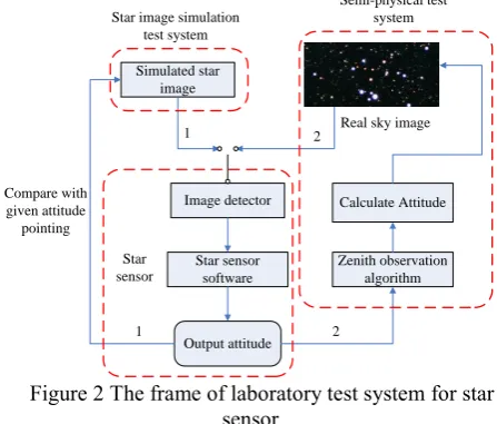
II. THE PRINCIPLE OF THE LABORATORY TEST SYSTEM Before we design the Laboratory test system, we should know the principle of star sensor. The star sensor is composed of the optical system and the electronic processing system. The optical system is composed of the lens, the CCD (or APS) detector plane and the baffle. It takes the photos from the real sky. The electronic processing system received the digital information of the picture from the optical system, and then used the software to calculate the attitude of the spacecraft. It included the star position estimation model, the star recognition model, the attitude determination model and the tracking model. The software flow of the star sensor is shown in Figure 1.
Image detector
Star position estimation
Star recognition
Attitude
determination Output attitude Star tracking
Algorithm Calculate Attitude
Lost in space acquisition
mode
Tracking mode Optical system
Figure 1 Software process flow of the star sensor From the Fig. 1, the star sensor uses the optical system to capture stars from the real sky firstly. Then, it uses the star position estimation model to calculate the star positions on the CCD plane. The star recognition method is used to identify the stars from star image. It matches the pattern constructed by the stars in the real star image with a catalog of reference stars pattern stored onboard to complete the identification. Finally, the attitude determination model uses the indentified star vectors to calculate the attitude of spacecraft. A star sensor usually operates in two modes: The Lost in Space Acquisition (LISA) mode and tracking mode. The difference between these two modes is whether a prior attitude is provided. In the LISA mode, star sensor uses the star recognition algorithm to get the initial attitude. When the initial attitude is given, the star sensor enters the tracking mode.
After the star sensor software and hardware design is completed, it is necessary to establish a laboratory test system to test the performance of the star sensor. From the Fig. 1, it is seen that the input of the star sensor is the star image. So the key point of the laboratory test system is provided a star image with known attitude pointing. The principle of the laboratory test system is described in Figure 2.
Image detector
Star sensor software
Output attitude
Zenith observation algorithm Calculate Attitude Compare with
given attitude pointing
Simulated star image
Real sky image
1 2
1 2
Star image simulation test system
Semi-physical test system
Star sensor
Figure 2 The frame of laboratory test system for star sensor
From the Fig. 2, we can see that the laboratory test system includes two parts, the star image simulation and
semi-physical test system. Star image simulation test system can provide simulated images in random directions with given attitude. Then the star sensor process the simulated star images and calculates the attitude of them. Compared the given attitude and the calculated attitude, we can test the star recognition rates of the star sensor. The semi-physical test system is designed for night sky experiments of the star sensor. Night sky experiments usually use the high accuracy telescope to point one direction and fixed the star sensor on it to calculate the attitude of the direction pointed by telescope. The semi-physical test system can test the accuracy of the star sensor. Under the condition of without telescope, we proposed a new zenith observation method to test the accuracy of star sensor.
Ⅲ. STAR IMAGE SIMULATION TEST SYSTEM
The star image simulation test system aims to provide star images under given attitude pointing. It consists of four main parts, searching star catalog, coordinate transformation, star magnitude simulation and the noise simulation part. The frame of the star image simulation is shown in Figure. 3.
Given attitude
Search the Stars in the
FOV
Map the stars coordinate from celestial to CCD plane
Add noise and disturbance of enviroment
Display simulated star
image
CCD noise nubela Moon lights Fast access star catalog
algorithm
Star magnitude simulation Load the star
catalog Pre-process the star catalog
Figure 3 The frame of star image simulation A. Star catalog accessing algorithm
APS sensor, we should set a magnitude limit to an appropriate value to ensure all selected guide stars can be imaged by the sensor and also can reduce the number of guide stars in the subset catalog [9].
In order to enhance the speed of the accessing star catalog, we divided the celestial sphere into several blocks in declination direction. In this paper, the size of FOV is 1212. So we selected the interval of block size is 3 and the whole celestial sphere is divided into (90-(-90))/3=60 blocks. If we give a random attitude pointing, the searching range of declination just occupies 5 blocks. So the speed of searching the star catalog is 1/12 of traditional searching range. Because the circle of right ascension is not evenly, we propose a method to calculate the range of right ascension when we know the declination and the size of FOV.
Suppose the random attitude pointing is (CJ0,CW0) at
right ascension and declination respectively. The half size of FOV is R degree. Then the range of declination is CW
(CW0R C, W0R). The right ascension calculation is not
simple like that. The range of right ascension increases along with the declination grows. So we use the upper limit of the declination CW0R to calculate the upper
limit of right ascension. The calculation range of right ascension is described in Figure 4.
U
V W
O Z
Cw0
ө
Cw0+R
A
B C
Figure 4 The calculation range of right ascension The range of right ascension can be calculated as follows:
0 0 0 0
( arctan(tan / cos( )), arctan(tan / cos( )) )
J J w J w
C C C R C C R (1)
The criterion of stars in the FOV is given as follows:
(
1, 2
)
(
1, 2
)
arccos(
) (
1, 2
)
i J
i W
C
i
n
C
i
n
i p
R
i
n
i p
(2)
where (
i,
i ) is guide star‟s right ascension and declination. n is the number of guide stars in the 5 blocks.p
is the boresight reference vector in celestial coordinate.i
is the guide stars reference vectors in celestial coordinate. R is the half size of FOV. (
) is thedot product operation.
is the separation angular distance between boresight vector and guide star vector.Firstly, we use the range of declination to determine which 5 blocks (sub catalog) should be searched, suppose n stars in these 5 blocks. Secondly, using the dot product in equation (2) between boresight reference vector
p
and n stars‟ vector to determine which star is in FOV. If n stars are all operated in dot product, it is time-consuming. We use the range of right ascension given by equation (1) to further reduce the number of stars searched in star catalog. The method can accelerate the speed of the accessing star catalog.B. Coordinate transformation
The simulated star image needs to calculate the guide star positions on the 2-D CCD plane. So the coordinate transformation is the first task of star image simulation. The guide star position in the celestial sphere is given by
i (right ascension) and
i (declination) (from the SKYMAP catalog). This position is in the celestial coordinate system (CCS), which is centered of the earth. The X-axis points at the mean equinox. The Z-axis points at the celestial pole. The Y-axis is constructed the right-hand system with the X and Z-axis. The guide star vector given by
i and
i can be transformed into the 3D coordinate in CCS and can be shown as [10]:[ , ,
U V W
]
T
[cos
icos
i, sin
isin
i, sin
i]
T (3) Guide star positions on the CCD coordinate system are needed. The center of the CCD coordinate system is the lens focus. The Z-axis points at the boresight direction of the star sensor. The X-axis is parallel to the rows direction of pixels of the CCD plane. The Y-axis is also constructed the right-hand system with the X and Z-axis. The guide star positions [X,Y,Z] in CCD coordinate system is given by [11]:
[ , , ]
X Y Z
T
M U V W
[ , ,
]
T (4) The matrix M is the rotation matrix from CCS to the CCD coordinate. A 3-2-1 Euler angle rotation is adopted. It rotates an angle
round the Z-axis first. Then rotating an angle
round the Y-axis and finally rotating an angle
round the X-axis. The frame of coordinate transformation is shown in Figure 5.U
V W
X Z
O α
δ Y
P S
Figure 5 The frame of coordinate transformation After the 3-2-1 rotating, we can get the rotation matrix M as follows [11]:
cos cos cos sin sin sin cos sin sin cos sin cos cos sin cos cos sin sin sin sin cos cos sin sin sin sin cos cos cos 1 0 0 0 cos sin 0 sin cos cos 0 sin 0 1 0 sin 0 cos cos sin 0 sin cos 0 0 0 1 M (5)
where
,
,
substituting equation (3) and (5) into (4), yields
sin sin cos cos cos( )
sin sin cos( ) cos cos sin( ) sin cos sin cos
cos sin cos( ) sin cos sin( ) cos cos sin
i i i
i i i
i i
i i i
i
X
Y
Z
(6)
Normalizing the equation (6), we can get the guide star position [x,y] on the 2-D CCD plane.
1
2
tan(
/ 2)
Y
x
f
X
Z
y
f
X
n
f
FOV
(7)where the f is the lens focus, FOV is the size of field of view (in this paper is 1212). n is the row or column number of pixels of CCD. Through the equation (7), we can get the star position on the 2D CCD plane to generate the simulated star image.
C. Star magnitude simulation
Star magnitude is important information on simulated star image. The visible magnitude of the stars is given by the SKYMAP catalog. The magnitude of stars is close related with the irradiance of stars and can be calculated as follows [12]:
0
2.51lg
ii
E
m
E
(8)where
E
0 is the irradiance energy of star with magnitude 0,E
i is the irradiance energy of star i,m
i is the magnitude of star i.If we want simulate magnitude 0~6.5, the irradiance difference ratio between magnitude 0 and 6.5 should larger than 100. But the computer gray level is limited and can‟t reach the 100 ratio. We use the linear relationship between magnitude and gray level to simulate the magnitude of stars and are given as follows:
G
i
10 (
m
max
m
i)
G
min (9)where
m
max is the maximum magnitude can be simulated (in this paperm
max
6.5
),G
minis the gray value according to them
max(G
min
(120 ~ 160)
),m
i is the magnitude of star i,G
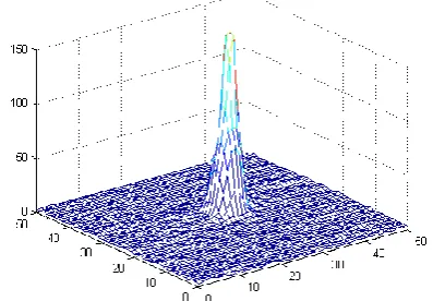
iis the gray value of star i.After getting the simulated gray value of star, we should consider the distribution of star energy. If the star energy concentrate on one single pixel, then we can‟t use the centroid algorithm to calculate subpixel accuracy star position. So the star sensor camera should be defocused slightly in order to spread the starlight energy over several neighbor pixels. If a small displacement
Z from the image plane, the star energy distribution area will increase and its diameter is [13]:
#
ZD
F
(10)where the F# is the optics number of the image sensor. The unit of the D is
m
.After defocusing, the starlight signal intensity distribution spread point function is reasonable approximated by the Gaussian function and the 2-D situation function can be written as [14]:
2 2
2 2
(
)
(
)
( , )
exp[
]
2
2
k
x
x
cy
y
cf x y
(11)where (x, y) is the valid neighbor pixels positions, (xc, yc)
is the accuracy star position on the CCD plane,
is the dispersion radius of the star intensity. Figure 6 is the simulation of single star point under consideration of defocus and Gaussian energy distribution.Figure 6 Star point simulation under 7×7 diameter
D. Noise and Sky environment simulation
Actually, the star image can be completed by the former three parts. In order to provide the noisy star image to test the stability of star sensor, we take full consideration of noise and sky environment effects in the star image simulation.
Nebula and Cluster is also a disturbance factor which can influence the operation of star sensor. Once the nebula or the cluster enters into the FOV, it will cover some useful stars because of its diameter is much bigger than single star. The Messier catalog [15] provides the information about the nebula and the cluster in the sky. There are about 110 nebulas in the sky, but only 35 nebulas can be detected by the CCD detector. The Messier catalog gives out the position and diameter of the nebulas.
First, we can calculate the number of occupied pixels per degree. The CCD size is 512×512 pixels, the FOV is
1212, then the occupied pixels per degree is calculated as follows:
512 25
25
(12 / 2)
(1 / 2)
P
(12)
P=64 pixels/degree
The Messier catalog give out the diameter of the nebula, suppose one nebula width is W and Height is H, then the apparent diameter of the nebula in image is:
_
(
/ 60) 64
_
/ 60
64
Row size
W
Column size
(
H
)
(13)where the Row_size and Column_size are the number of pixels occupied by the nebula on CCD plane.
The moon lights entering the FOV is also taken into account, it can be simulated by circle or ellipse shape.
Ⅳ. ZENITH OBSERVATION ALGORITHM
The star image simulation test system is described above. It just can test the star recognition rates and the software stability of the star sensor. It is necessary to design the semi-physical test system to test the accuracy of the star sensor. The semi-physical test system captured the stars from the real night sky. Night sky experiments usually use the high accuracy telescope to point one direction and fixed the star sensor on it to calculate the attitude of the direction pointed by the telescope. Under the condition of without telescope, we proposed a new zenith observation method to test the accuracy of star sensor.
The zenith method takes the earth as an evenly rotational turntable. It needs high accuracy spirit level to make sure the star sensor points at the zenith direction. The star sensor captured the stars from the zenith direction and calculated the attitude. Then, we use the astronomy knowledge to figure out the zenith position at the shooting time. Compared the star sensor‟s attitude with the zenith ideal attitude, we can test the accuracy of the star sensor without telescope.
Before using the zenith method, we should know two input parameters, the shooting time (UTC) and the location of star sensor (geographical latitude, geographical longitude and geographical Height in geocentric coordinate system). The output is the zenith position in the conventional inertial system. The flow of the coordinate transformation is described in Figure 7.
UTC (Coordinated Universal Time) to JD
(Julian Day)
UTC’MJD to TDB’s MJD
TDB’s MJD to TDB’s JD JD to MJD( Modified
Julian Day)
Terrestrial system to Conventional Terrestrial
system Celestial System to
Terrestrial system
Celestial System to Conventional Inertial System
Conventional Inertial System to (CIS,J2000)Conventional Terrestrial system(CTS,ECF)
Coordinate transformation Observation Time and
Position
Figure 7 The flow of Zenith observation algorithm The zenith observation algorithm also can be written by [16]:
[
CIS
]
Q t R t W t CTS S t
( ) ( )
( )[
] ( )
(14) CIS: Conventional Inertial SystemCTS: Conventional Terrestrial System
S(t): the transformation matrix from the geocentric coordinate system to CTS.
W(t): the transformation matrix from CTS to Terrestrial System (TS) consideration of the polar motion effects
R(t): the transformation matrix from TS to Celestial System (CS), from the rotation of the Earth around the axis of the pole.
Q(t): the transformation matrix from CS to CIS under consideration of the precession and nutation.
The matrix described above needs a lot of observation information released by International Astronomical Union (IAU) every year, and the calculating doesn‟t mention in detail in this paper.
Ⅴ. EXPERIMENTS AND RESULTS
In this section, we design a number of experiments to verify the laboratory test system designed in this paper. The experiments are divided into two parts, the simulated star image test and the semi-physical test.
A. Simulated star image test
Star image simulation uses the software to simulate the star image captured by the CCD sensor. The theory of the star image simulation is described in the section Ⅲ. With
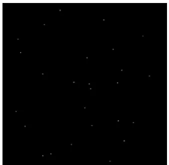
Figure 8 Original star image simulation without noise pointing at (-130,-60,90)
In Fig. 8, the star image pointing at the (-130,-60,90) is simulated. It is shown that the simulated star image method is validated and can be used to test the star sensor.
Figure 9 Noisy star image simulation with adding white Gaussian noise
In Fig. 9, the white Gaussian noise is added into the simulated star image. It can used to test the stability of star sensor software.
Figure 10 The nebula simulation in the simulated star image
In Fig. 10, the nebula is simulated in the star image. The nebula is M33 (in the Messier catalog) with position at (23.475, 30.65), so the boresight of the star sensor is selected at (26,33,90). This simulation is considered the sky environment effects on star sensor operation.
Figure 11 The moon lights entering FOV simulation In Fig. 11, we simulated the moon lights entering into the star sensor FOV. The moon can affect the operation of the star sensor. The simulation can test the star recognition rate, when the star sensor under the stray light entering into the FOV.
We also selected 1000 random attitudes adding white Gaussian noise on star magnitude from 0.1 to 0.6 to test the performance of star sensor. It took 0.4 second to complete one image processing and the star identification success rate under the noise lower than 0.3 magnitude was 98.6%. Once the LISA is success, the star sensor can enter the tracking mode quickly. When the magnitude higher than 0.4, the success rate of star recognition has a little decrease. The experiments results showed that the star sensor software was stable and insensitive to the magnitude noise. It also demonstrated that the star image simulation test system is feasible.
B. Semi-physical experiments
Except the simulated star image test, we also take experiments in real night sky. The night sky experiments were carried out on NAOC‟s observation station in XingLong, Hebei Province, in December 2009. We took about 900 images under different orientations and different noises. A real sky image captured by the star sensor and its 3D processing is given in Figure 12 and 13.
Table 1 The data using zenith method to test the accuracy of star sensor
Index Photo time Ideal RA Ideal Declination Calculated RA Calculated Dec IMG_599 2009 12 14 22 54 47 64.50938087 40.18066423 64.7728172 40.45749233 IMG_600 2009 12 14 22 54 51 64.52608685 40.18067916 64.7909947 40.45777087 IMG_601 2009 12 14 22 54 55 64.542793 40.1806941 64.80881278 40.45855001 IMG_602 2009 12 14 22 55 0 64.56367565 40.18071278 64.82680278 40.45757764 IMG_603 2009 12 14 22 55 4 64.58038164 40.18072773 64.84569346 40.45808776
…
… … …
…
…
…
…
IMG_660 2009 12 14 22 59 43 65.74563994 40.1817753 66.014071 40.46061216 IMG_661 2009 12 14 22 59 48 65.76652276 40.18179417 66.03273553 40.46010127 IMG_662 2009 12 14 22 59 53 65.78740575 40.18181304 66.0537399 40.4601582 IMG_663 2009 12 14 22 59 58 65.80828874 40.18183191 66.07607295 40.46018708 IMG_664 2009 12 14 23 0 3 65.82917174 40.18185079 66.09627866 40.45950718
Figure 13 The 3D process of the real sky image There are about 100 images pointing at the zenith in all real sky images. We selected 66 images to validate the zenith observation method and to test the relative accuracy of the star sensor. The ideal attitude figured out by the zenith method and the calculated attitudes provided by the star sensor about the 66 images are shown in table 1.
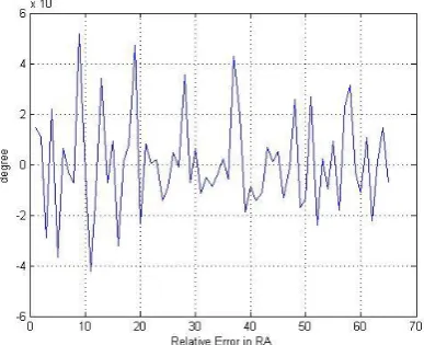
We can calculate the relative accuracy of the star sensor. The relative error in right ascension and declination are shown in Figure 14 and 15.
Figure 14 The relative attitude Error in Right Ascension
In Fig. 14, we can calculate the relative attitude error in right ascension using the data in table 1. The star sensor accuracy in right ascension is about
3
5 10 3600 18 .
Figure 15 The relative attitude Error in Declination In Fig. 15, we also can calculate the relative attitude error in Declination through the data in table 1. The star sensor accuracy in declination direction is about
3
9 10 360032.
Through the experiments above, we can see that the zenith method can meet the accuracy testing requirements of the star sensor without telescope. The laboratory test system designed in this paper is proved to be feasible and can meet the requirements of performance evaluation of the star sensor.
Ⅵ. CONCLUSIONS
test the relative accuracy of the star sensor without using telescope. Experiments results prove our Laboratory test system is feasible and can meet the requirements of performance evaluation of the star sensor.
REFERENCES
[1] C.C. Liebe. “Star trackers for attitude determination,”. IEEE Aerospace and Electronic Systems Magazine, 10 1995, pp. 10-16.
[2] W. James Alexander, H. Daniel Chang, “Cassini Star Tracking and Identification Algorithms, Scene Simulation, and Testing,” SPIE, vol. 2803, pp. 331-336, 1996. [3] J. Leif Jorgensen, A. Pickles. “Fast and robust pointing and
tracking using a second generation star tracker,” SPIE, vol. 3351, pp. 51-61, 1998.
[4] J. Gwanghyeok. “Autonomous star sensing, pattern identification, and attitude determination for spacecraft: an analytical and experimental study,” Doctor thesis, Texas A&M university, 2001.
[5] P. oosthuizen, C. Collingwood, L. Saleem, C. Alexander and G. Scott. “Development and on-orbit results of the SSTL low cost commercial star tracker,” AIAA Guidance, Navigation and Control conference and exhibit, 2006, pp. 1-11.
[6] W. zhao-kui, Z. yun-lin. “Design and implementation of star pattern simulator for use of space surveillance,” Journal of System Simulation. Vol.18 (5), pp. 1195-1211, 2006.
[7] H. yi-ning, G. Yan. “Design and realization of a dynamic display algorithm for star map,” Journal of Astronautics, Vol.29(3), pp. 849-853, 2008.
[8] R. Giancarlo. M. Antonio. “Laboratory test system for performance evaluation of advanced star trackers,” J Guid Control DYN 25(2), pp. 200-208, 2002.
[9] J. Jiang, G. J. Zhang, X. G. Wei, X. Li, “Rapid star tracking algorithm for star tracker,” IEEE Aerospace and Electronic Systems Magazine, vol. 24, pp.23-33, 2009. [10]J. Yang, T, Zhang, J.Y, Song, B, Liang, Q,Q, Ding. “The
Algorithm Research of Ground Celestial Sphere and Dynamic Star Simulator”, Journal of system simulation, Vol.22, pp. 202-206, 2010.
[11]Z. jun-ping, L. Tao, Z. jian-lin and Q. guo-hui. “A method of CCD star image simulation,” Chinese space science and technology, Vol.3, pp. 46-50, 1999.
[12]C. Harry strunz, B. Troy and D. ethridge. “Estimation of stellar instrument magnitudes,” SPIE, vol.1949, pp. 228-235, 1993.
[13]G. Rufino, D. Accardo. “Enhancement of the centroiding algorithm for star tracker measure refinement,” Acta Astronaut, vol.53, pp.135-147., 2003.
[14]Katake, A.B. “Modeling, image processing and attitude estimation of high speed star sensors,” Doctor thesis, Texas A&M university, pp.33-37, 2006.
[15]http://202.112.85.100/aobn/resource.htm (accessed on 9 October 2010).
[16]http://www.iers.org/nn_11216/SharedDocs/Publikationen/ EN/IERS/Publications/tn/TechnNote32/tn32,templateId=ra w,property=publicationFile.pdf/tn32.pdf (accessed on 30 June 2010).
Jun yang and is currently a Ph.D. candidate in the Department of Automation at Tsinghua University. He has received his B.S. degree in automation from
Northwestern Polytechnical University, China, in 2004, received Master from Beijign University of Posts and Telecommunications in 2007. His research interests include star sensor technology, Micro-Satellite technology and artificial intelligence.
Bin Liang is a Professor in the Department of Automation at Tsinghua University. He received his Ph.D. degree in Precision Instrumentation and Machinery from Tsinghua University, China, in 1994. His research interests include Micro-Satellite technology and space robotics.
Tao Zhang is an Associate Professor in the Department of Automation at Tsinghua University. He received his B.S., M.S. and Ph.D. degrees in Electrical Engineering from Tsinghua University, China, in 1993, 1995 and 1999, respectively. He received his second Ph.D. degree in Electrical Engineering from Saga University, Japan in 2002. His research interests include robotics and system control engineering.
Jing-yan Song is a Professor in the Department of Automation at Tsinghua University. He received his Ph.D. degree in Systems Engineering and Engineering Management from The Chinese University of Hong Kong, China, in 1998. His research interests include Micro-Satellite technology, intelligent transportation system and space robotics.

![Figure 7 The flow of Zenith observation algorithm The zenith observation algorithm also can be written by [16]:](https://thumb-us.123doks.com/thumbv2/123dok_us/7825521.1665936/5.595.335.508.84.222/figure-zenith-observation-algorithm-zenith-observation-algorithm-written.webp)