Analysis of Wind Turbine Pressure Distribution and 3D Flows Visualization on Rotating Condition

ISSN (e): 2250-3021, ISSN (p): 2278-8719

Vol. 06, Issue 02 (February. 2016), ||V1|| PP 18-30

Analysis of Wind Turbine Pressure Distribution and 3D Flows

Visualization on Rotating Condition

Tinnapob Phengpom

, Yasunari Kamada

, Takao Maeda

,

Tasuku Matsuno

and Noriaki Sugimoto

1

(Division of System Engineering, Mie University, Japan)

2,3_{(Division of Mechanical Engineering, Mie University, Japan)} 4,5_{(Graduate school of Engineering, Mie University, Japan)}

Abstract: - Rotational effects influence the aerodynamic performance of wind turbine rotor severely. The

objective of this research attempted to study the rotational effects in the vicinity of the wind turbine blade surface. Detailed flow measurements on wind turbine blade were performed in a wind tunnel. The test wind turbine has a three-bladed rotor with a radius of 1.2m. Each blade is twisted and tapered as same as commercial wind turbine blade. The maximum power coefficient of the test wind turbine is 0.43 at the tip speed ratio of 5.2. The measured velocities around blade section were detected using a Laser Doppler Velocimetry (LDV) while the pressure distributions on blade surface were detected using 32 pressure sensors for the rotating condition. All experiments were conducted for an optimum tip speed ratio. As a result, it is clarified that the rotational effects appear obviously on the inboard of the blade. The axial and tangential velocity components indicate strong velocity gradients on the leading edge and trailing edge. The rotational effects increase the sectional lift force and delays transition point in the inboard.

Keywords: - Wind turbine, Pressure distribution, LDV, Three-dimensional flows, Aerodynamic forces

I.

INTRODUCTION

Global Wind Energy Council (GWEC) reported that wind power is the most reliable renewable energy technology. The wind power has the advantages of high energy conversion rate, large industrial scale, and high social benefits [1]. German aerodynamicist Albert Betz proposed the maximum wind turbine coefficient of 16/27 which is known as “the Betz limit” [2]. Insight understanding of aerodynamic behavior is the key factor in determining the higher efficiency of the wind turbine rotors. Much research on the wind energy carrying out for the last few decades have afforded to improve the wind turbine efficiency as close to the Betz limit. Rozenn, W. et al attempted to study the influence of the wind speed profile comparing data with numerical prediction using Blade Element Momentum Theory (BEMT) in order to increase wind turbine rotor performance. The result showed the difference between measurements and numerical prediction due to 3D complicated flows on a rotating condition [3]. Rosten, G. reported the results of pressure distributions on wind turbine rotor in the wind tunnel. The pressure distributions detected during non-rotating and rotating operations. The results showed that rotational effects lead to stall delay and lift enhancement at the inboard [4]. Wood, D. et al explained a stall delay in terms of pressure depends on the local solidity of the blades and changes to the external inviscid flow [5]. Schreck, S. et al examined surface pressure measurements from the NREL UAE Phase VI experiment and noted that rotational augmentation is connected to radial surface pressure gradients [6]. Sicot, C. et al investigated an experimental study on a small wind turbine and compared sectional surface pressure distributions from a non-rotating blade and a rotating operating in turbulent flow. The result observed that the blade root region presented enhanced lift, but no evidence of stall delay was observed [7].

In addition, the rotational effects also have influence severely on the velocity flow phenomenon. Martínez, G.G. et al presented a three-dimensional velocity profile in the boundary layer of a rotating blade. The results showed the effect of three-dimensional flow changes the boundary layer velocity profile around the blade surface, and delay flow separation [8]. Dua, Z. et al also presented the rotational effects on the blade boundary layer. The results showed that 3D flow condition had a general impact on separation as compared with 2D conditions. A radial flow plays a significant role in the 3D stall delay [9]. Our previous research succeeds to measure the three-dimensional velocity using an LDV measurement [10, 11]. The velocity field around the rotating blade showed high acceleration area on the leading part of the blade suction surface. The skin friction coefficient for low tip speed case is higher than that of the optimum case because leading part has strong shear near the surface. The circulation strength around the blade for optimum operation shows bigger value than that of the stall except near the blade root.

generalized study results as a power coefficient that is obtained from test wind turbine, pressure distribution, velocity distribution on the rotating condition.

II.

NOTATIONS

Nomenclature Ue : Velocity at outer edge of boundary layer [m/s]

Ad : Rotor swept area [m

2

] Uref : Inflow velocity [m/s]

a : Axial induced factor [-] u : Axial velocity component [m/s]

a : Tangential induced factor [-] u1 : u1 velocity component from 1st probe [m/s]

CL : Lift coefficient [-] u2 : u2 velocity component from 1st probe [m/s]

Cp_Xfoil : Pressure coefficient from Xfoil [-] u3 : u3 velocity component from 2nd probe [m/s]

Cp_LDV : Pressure coefficient from LDV [-] v : Tangential velocity component [m/s]

Cp_tap : Pressure coefficient from pressure tap [-] w : Radial velocity component [m/s]

Cpow : Power coefficient [-] x : Axial position [m]

c : Local chord length [mm] y : Chord position [m]

L : Sectional lift [N] Greek symbols

N : Numbering of pressure tap [-] α : Angle of attack [°]

P : Power [W] λ : Tip speed ratio (=RΩ/U0) [-]

p0 : Static pressure of mainstream wind [Pa] Ψ : Azimuth angle [°]

pd : Dynamic pressure of inflow wind [Pa] β : Pitch angle [°]

pi : Local static pressure at pressure tap [Pa] θtwist : Twist angle [°]

Q : Torque [Nm] θ1 : Tilted angle between u1 and rotor axis [°]

R : Blade radius (=1.2) [m] θ2 : Tilted angle between u2 and rotor axis [°]

r : Local blade radius [m] θ3 : Tilted angle between 2nd probe and rotor axis [°]

si : Measurement taps distance connecting ρ : Density of air [kg/m3]

midpoint of tap adjacent to each other in Ω : Angular velocity [1/s]

blade section [m] Г : Circulation [m2/s]

U0 : Mainstream velocity (=7.0) [m/s] _i : Tilted angle between pressure measurement tap

and chord line [°]

III.

EXPERIMENT

APARATUS

AND

METHOD

3.1 The blade design

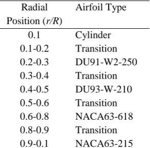
This research focused on the horizontal axis wind turbine. A test wind turbine has a three-bladed rotor with a radius of 1.2 m. The test blades for this experiment were made from Polyurethane. The test blade is twisted and tapered blade design using the Blade Element Momentum Theory (BEMT) like commercial wind turbines that have thick airfoil at the inboard and thin airfoil at the outboard. The blade shape was designed using four different airfoils (DU91-W2-250, DU93-W-210, NACA63-618, and NACA63-215). These airfoils

were set in the radial position as shown in Table 1. The root cut out is radial position r/R = 0.1 where section is a

cylinder with diameter 70 mm. Four airfoils smoothly connected and distributed along the blade in a span-wise

direction. The blade ended at radial position r/R=1.0 with chord length 85 mm of NACA63-215. Figure 1 shows

the plan form and twist distribution of test blade. Blue and red lines indicate leading edge and trailing edge

positions for each radial position r/R. Green line indicates the twist angle. The maximum twist angle θtwist =

18.33[°] was set at radial position r/R= 0.2 and decreased until the twist angle θtwist = 0 [°] at radial position r/R

3.2 Wind tunnel measurements

Figure 2 shows a schematic view of experimental apparatus for this experiment. The test wind turbine was set in the wind tunnel. The test section of the wind tunnel is an opened section with a diameter of 3.6 m, and a length of 4.5 m. The sectional corrector size is 4.5x4.5 m. The distance from rotor plane to wind tunnel air outlet is 1.85 m. The mainstream flow is driven by a 400 kW variable speed fan set at the return passage. The mainstream speed is measured by a Pitot-tube, and the thermometer is installed to measure air temperature. The maximum velocity can be achieved in the high-speed velocity of 30 m/s. The experiment is conducted at a

constant mainstream velocity U0 of 7 m/s. The turbulence intensity is less than 0.5%. The wind turbine rotation

could be controlled by using a servomotor. The mechanical power is measured through a torque meter and rotational speed sensor. During the measurements, the wind turbine rotor axis was set at mainstream direction.

Generally, the flow field around wind turbine at the maximum efficiency point expands in the wake until 1.22 times of the rotor diameter. It is considered that the wind turbine wake should be in the uniform wind speed area of the test tunnel. The radius in test rotor is 1.2m, so the radius of wind turbine wake expand up to 1.47m in optimum operation. In this case the radius of uniform wind is 1.7m for this wind tunnel. Thus, the flow affected by wind turbine rotor can stay in the uniform wind.

Radial

Position (r/R)

Airfoil Type

0.1 Cylinder

0.1-0.2 Transition

0.2-0.3 DU91-W2-250

0.3-0.4 Transition

0.4-0.5 DU93-W-210

0.5-0.6 Transition

0.6-0.8 NACA63-618

0.8-0.9 Transition

0.9-0.1 NACA63-215

Table 1. Airfoil type distribution

0.1 0.2 0.3 0.4 0.5 0.6 0.7 0.8 0.9 1.0

Leading Edge Trailing Edge Twist Angle

0.1 0.2 0.3 0.4 0.5 0.6 0.7 0.8 0.9 1.0

30 20 10 0

0 50 100

-50

-100

-150

C

h

o

rd

-wis

e

p

o

sitio

n

[mm]

T

wis

t a

n

g

le

θtwist

[

°]

Fig. 1 Test blade plan form

Radial position r/R [-]

Fig. 2 Experimental setup for the wind tunnel test of the HAWT model

3.2.1 Pressure measurement on the blade section

In this section, the pressure measurement using the pressure sensors will be presented. These experiments were carried out in a wind tunnel to detect the surface pressure distribution along the blade span in the rotating condition.

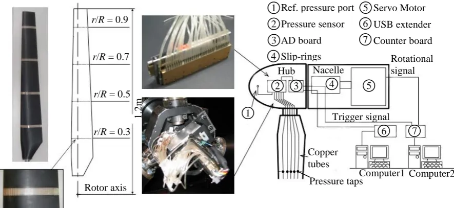
Figure 3 shows the span-wise position of measurement section, the pressure measuring system and the diagram of the system. As shown in Fig. 3, the pressure taps are perpendicularly set to the pitch axis at radial

positions r/R = 0.3, 0.5, 0.7 and 0.9. Each tap has a diameter of 0.4 mm. The pressure sensors are of a

semiconductor type, having 32 measuring and one reference ports. Theses sensors have a rated pressure of ±7.65kPa. The pressure sensors are installed in the hub, and the pressure membrane is parallel to the rotating surface in order to avoid the error due to centrifugal forces. The static pressures data at each pressure tap can be passed to the pressure sensors through the pressure transmission tubes as analog signals in the A/D board in the rotating system, and after being converted into digital signals are transmitted through the slip rings in the main axis to a personal computer for processing. The sampling time for one measurement tap is 0.1 ms. Thus, the sampling time for 32 pressure taps is 3.2 ms. The pressure data are averaged from 100 revolutions of the wind turbine rotor.

Figures 4 (a)-(d) show the position pressure taps at radial positions r/R = 0.3, 0.5, 0.7 and 0.9. The

pressure taps are small holes drilled perpendicular to the blade surface. The density of pressure tap is high near the leading edge and low near the trailing edge. Because the pressure transition on the airfoil surface is sharp

U0

3

.6

m

Wind tunnel outlet

Tower Nacelle

Base Rotor

4.5 m

4

.5

m

Inlet

R

=

1

.2

m

1.85 m Pitot tube

0.15 m Thermometer

Inlet Outlet

4.5 m Fan

Open measurement section 9.5

m

U0

31 m

Fig. 3 Pressure measuring system and control system. 1

Hub

2 3 4 5

6 Nacelle

7 Rotational signal 1

Trigger signal 2

3

4

5

6

7 Ref. pressure port

Pressure sensor

AD board

Slip-rings

Servo Motor

USB extender

Counter board

Computer1 Computer2 Pressure taps

Copper tubes

1

.2

m

r/R = 0.3

r/R = 0.7

r/R = 0.5

r/R = 0.9

T h ick n ess x / c [ -]

Fig. 4 (a) Position of pressure taps

(DU91-W2-250, r/R = 0.3, c = 139.6x10-3m)

Chord-wise position y/c [-]

0.0 0.2 0.4 0.6 0.8 1.0 Pressure taps 0.5 0.3 0.1 -0.1 -0.3 -0.5

-Fig. 4 (b) Position of pressure taps

(DU93-W-210, r/R = 0.5, c = 124x10-3m)

Chord-wise position y/c [-]

0.0 0.2 0.4 0.6 0.8 1.0 Pressure taps 0.5 0.3 0.1 -0.1 -0.3 -0.5 -T h ick n ess x / c [ -] Pressure taps

Fig. 4 (c) Position of pressure taps

(NACA63-618, r/R = 0.7, c = 108.4x10-3m)

Chord-wise position y/c [-]

0.0 0.2 0.4 0.6 0.8 1.0 0.5 0.3 0.1 -0.1 -0.3 -0.5 -T h ick n ess x / c [ -]

Fig. 4 (d) Position of pressure taps

(NACA63-215, r/R = 0.9, c = 92.8x10-3m)

Chord-wise position y/c [-]

0.0 0.2 0.4 0.6 0.8 1.0 0.5 0.3 0.1 -0.1 -0.3 -0.5 -Pressure taps T h ick n ess x / c [ -]

near the leading edge. The pressure values at trailing edge can be estimated by the tendency of the pressure gradient.

3.2.2 Three-dimensional velocity measurement on the blade sections

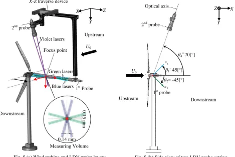
Figure 5 (a) presents the LDV system and the wind turbine placement. A Laser Doppler Velocimetry (LDV) measurement was carried out for detecting three-dimensional velocity components in the vicinity of the wind turbine blade surface. To detect local three-dimensional velocity components, two LDV probes were set and three pairs of laser beams were applied. The coincidence mode for each velocity components was chosen to minimize the measuring volume. This measurement was set three-dimensional Cartesian coordinate system. The

measuring volume was fixed at the rotor axis height. The two probes were set on the X-Z traversing device.

Therefore, the measuring volume position could be changed according to both axial and radial positions. The

number of samples was 1.0 x 105 for one local measuring point. The azimuth angle for each sample was

detected by single reset pulse for rotor orientation. A 0.1 degree azimuth BIN was applied for cyclic flow phenomena. Figures 5 (b) and (c) show the side view of the two LDV probe settings and the top view of the two

LDV probe settings, respectively. The 1st probe was set on a horizontal plane at rotor axis height. The 1st probe

was inclined θ3 = 10 [°] to rotor plane seeing from the top for avoiding interference by the blade itself. The focal

length of the 1st probe is 1,000 mm. The 1st probe was used to detect u1 and u2 velocity components. The

directions of u1 and u2 were at the angle θ1 = 45 [°] and θ2 = -45 [°] to the rotor axis. The 2nd probe was set

vertical seeing from upstream, and inclined θ4 = 70 [°] to the rotor axis. The focal length of the 2nd probe is

1,600 mm. The 2nd probe was used to detect the u3 velocity component in the radial direction. The u1, u2 and u3

velocity components are detected from the arrangement of the LDV probe. The measured velocities data have a

slight discrepancy from the designed airfoil section at radial position r/R due to azimuth position.

The u1, u2 and u3 velocity components can be converted to velocity components on the X, Y and Z axes

of the rotor blade that are defined as Eq. (1).

1 1 3 1 1 3

2 2 3 2 2 3

3

c o s c o s s i n c o s s i n

c o s c o s s i n c o s s i n

0 0 1

u u u v w u                  _                      (1)

Fig. 5 (a) Wind turbine and LDV probe layout Green lasers

Violet lasers

1st Probe

probe U0

Upstream

Focus point

2nd probe

Blue lasers

0

.1

5

mm

0.14 mm Measuring Volume Downstream

Z

Y X

X-Z traverse device

stand on the Y-axis and w is the radial velocity component that stand on the Z-axis.

The tilted angles θ1, θ2 and θ3 are substituted by 45 [°], -45 [°] and 10 [°], respectively. Thus, the

velocity conversion matrix can be expressed as Eq. (2).

1

2

3

0 .6 9 6 0 .7 0 7 0 .1 2 3

0 .6 9 6 0 .7 0 7 0 .1 2 3

0 0 1

u u

u v

w u

     

     

 

     

   

 

   

 

(2)

As shown in Eq. (2), the ingredients of each velocity component obtaining from the LDV probe

comprised breaking vectors of velocity components on the X, Y and Z axes. Thus, the axial, tangential and radial

velocity components can find from the property of inverse matrix as shown in Eq. (3).

1

2

3

0 .7 1 8 0 .7 1 8 0 .1 7 7

0 .7 0 7 0 .7 0 7 0

0 0 1

u u

v u

w u

  

   

 

   

  _{ }

   

     

     

(3)

Finally, the three-dimensional velocity components on the rotor coordinate are denoted by Eqs. (4), (5) and (6), respectively.

1 2 3

= 0 .7 1 8 + 0 .7 1 8 - 0 .1 7 7

u u u u (4)

1 2

= 0 .7 0 7 - 0 .7 0 7

v u u (5)

3

=

w u (6)

The measuring point is fixed at an azimuth angle of 270 [°]. The relative measuring point to the blade surface is detected by the rotor azimuth angle. The non-dimensional axial, tangential and radial velocity components on the suction are discussed.

Fig. 5 (b) Side view of two LDV probe setting Optical axis

2nd probe

1st probe

Upstream _Downstream

u₁

u₂

U0

θ4= 70[°]

θ2= -45[°]

θ1 =

45[°]

X

Upstream

Downstream

U0 Y

X

Z

1.0 m

1.6 m

Optical axis

1st probe

2nd probe

Optical axis Violet lasers

Fig. 5 (c) Top view of two LDV probe setting

u₃

θ3=10[ᵒ]

IV.

RESULTS

AND

DISCUSSION

4.1 Wind turbine performance

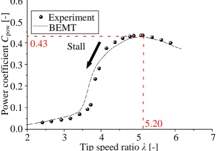
Figure 6 shows the power coefficient curve of the test wind turbine. The power coefficient is expressed as a function of the tip speed ratio. Normally, the power coefficient can be defined as Eq. (7).

p o w 3 3

d 0 d 0

0 .5 0 .5

P Q Ω

C

A U A U

  

 (7)

Where Cpow is the power coefficient, Q is the rotor torque, Ω is the angular velocity, ρ is the density of air, Ad is

the rotor swept area, P is the power output and U0 is the mainstream velocity. The tip speed ratio  is defined as

Eq. (8).

0

R Ω

U

  (8)

As shown in Fig. 6, the solid circle point indicates the measured power coefficient, and the line

indicates the estimated power coefficient from BEMT. The highest measured power coefficient is 0.43 at the tip

speed ratio λ = 5.2. The measured power coefficient Cpow at the optimum condition illustrates slightly greater

values than BEMT prediction.

Fig. 6 Power coefficient of wind turbine

Tip speed ratio λ [-]

2 3 4 5 6 7

Experiment 0.6

0.5

0.4

0.3

0.2

0.1

0.0

Po

wer

co

ef

ficien

t

Cpow

[

-]

BEMT

0.43

4.2 Pressure distribution on the blade surface

The pressure distribution at the inboard and outboard sections (r/R = 0.3 and 0.7) were investigated

comparing with the pressure coefficients from LDV measurement and numerical prediction as a function of

chord station y/c. The pressure on the rotating blade surface depends on the inflow velocity (Uref), local angle of

attack (α) and blade surface shape. Thus, the data were reduced by defining a non-dimensional parameter. The

pressure distribution is expressed in dimensionless form by the pressure coefficient.

The pressure coefficient Cp_tap was defined as the ratio between the surface pressure measured on the

blade section surface and the dynamic pressure of the sectional inflow wind, as indicated in eq. (9).

i 0 i 0

p _ t a p 2

d r e f

( ) ( )

0 .5

p p p p

C

p U

 

  (9)

Where pi is the static pressure at the tap, p0 is the reference static pressure, pd is the dynamic pressure of the

sectional inflow velocity and Uref is the sectional inflow velocity, which is defined as

 2

2

re f [ 0(1 ) ] (1 )

U  U a  Ω r a (10)

Where r is the local blade radius, a is the axial induced factor andais the tangential induced factor that are

calculated by BEMT with details of test blade and the wind turbine operational data.

The pressure coefficient also can be calculated from measured velocities. The pressure coefficient from

velocity measurement Cp_LDV can be derived as Eq. (11).

2 e p _ L D V

r e f

1 U

C

U

 

   

 

(11)

Where Ue is the relative velocity at the outer edge of the boundary layer.

Figures 7 (a) and (b) show the pressure distributions from the pressure measurement, velocity measurement and Xfoil [12] prediction. The solid green circle indicates the pressure coefficient from pressure

measurement Cp_tap. The solid red circle indicates the pressure coefficient from velocity measurement Cp_LDV.

The solid black line indicates the pressure coefficient from Xfoil prediction Cp_Xfoil. The pressure distribution

shows that the Cp_tap = 1.0 is at the stagnation point near the leading edge. And then, the Cp_tap on pressure

surface decreases. Cp_tap on the suction surface shows minimum near around the leading edge and then it rises as

close to the trailing edge. Finally, the Cp_tap recovers to a small positive value near the trailing edge.

As shown in Fig. 7 (a), the pressure coefficient Cp_Xfoil shows the difference from Cp_tap andCp_LDV. The

pressure coefficients Cp_tap and Cp_LDV were measured in rotating blade condition while the pressure coefficient

Cp_Xfoil was simulated in non-rotating condition from Xfoil software. Generally, the aerodynamic characteristics

extracted from the rotating blades commonly present evidence of rotational effects, such as stall delay and lift

enhancement. Especially, the radial positions are close to the blade root. The pressure coefficient Cp_Xfoil predicts

a transition point near the chord station y/c = 0.15 while transition points from the pressure tap and LDV

measurement delay to the chord station y/c = 0.3. For the chord station 0.15 < y/c < 0.5, the pressure coefficient

Cp_Xfoil increases rapidly while the pressure coefficients Cp_tap and Cp_LDV increase gradually. The pressure

coefficients Cp_tap and Cp_LDV show quite stable values which phenomena is known as a laminar separation

bubble at the chord station 0.25 < y/c < 0.3.

In Fig. 7 (b), the pressure coefficient Cp_Xfoil is very similar trend to Cp_tap and Cp_LDV. It seems that the

rotational effects can not affect the pressure distribution near the blade tip section The slope of the pressure

coefficients Cp_tap, Cp_LDV and Cp_Xfoil against chord position y/c clearly show approaching a zero slope at the

chord station of 0.4 < y/c < 0.5. Moreover, the pressure coefficients on this chord station region are not

significant difference values. It seems like the formation of a laminar separation bubble. The chord station y/c =

0.5 is presented as a transition point, and then the pressure coefficients are rapidly increased close to trailing

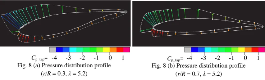
Figures 8 (a) and (b) show the measured pressure profile pattern around the blade section at radial

positions r/R = 0.3 and 0.7, respectively. The color bar indicates the value of local pressure coefficient Cp_tap. In

these figures, the colored arrows indicate the quantity and direction of the pressure coefficient in each pressure tap. Each arrow is perpendicular to the blade surface. The sign of arrow represents the direction of pressure. The arrow toward inside indicates a positive pressure while the arrow toward outside indicates a negative pressure. Total lift on the blade section depends on the difference between the pressure distribution profile on the upper surface (Suction surface) and the lower surface (Pressure surface). Generally, high negative pressure coefficient occurs on the leading edge of the suction surface and is gradually increased pressure approaching the trailing edge. While, high positive pressure coefficient occurs on the leading edge of pressure surface and is gradually decreased pressure approaching the trailing edge. The pressure distribution integrated around the blade section

provides sectional lift coefficient. The rotational effects influence the lift enhancement at radial position r/R =

0.3. Estimated sectional lift coefficients CL= 1.58 and 1.18 were obtained at the radial positions r/R = 0.3 and

0.7, respectively.

4.3 Flow field visualization on the blade sections

Figures 9 (a) and (b) show the sectional view of the axially induced velocity for the optimum tip speed

ratio at radial positions r/R = 0.3 and 0.7, respectively. The color bar shows the intensity of axially induced

velocity on the blade surface normalized with the mainstream velocity U0. The positive value indicates the

direction from upstream to downstream. As shown in Fig. 9 (a), the high positive induced velocity (u/U0)-1 >

1.5 is observed above the leading edge while the high negative induced velocity in the range of -1.5 < (u/U0)-1 <

-1.0 is observed above the chord station of 0.4 < y/c <1.0. As shown in Fig. 9 (b), the high induced velocity

(u/U0)-1 > 1.5 is observed at chord station of 0 < y/c < 0.1 while the high negative induced velocity (u/U0)1 <

-1.5 is observed at the chord station of 0.5 < y/c < 1.0.

This flow is strongly influenced by the blade itself, and strong velocity gradients can be observed at the leading edge and the trailing edge regions.

-4 -3 -2 -1 +0 +1

Cp_tap

=

Fig. 8 (a) Pressure distribution profile

(r/R = 0.3, λ = 5.2)

-4 -3 -2 -1 +0 +1

Cp_tap

=

Fig. 8 (b) Pressure distribution profile

(r/R = 0.7, λ = 5.2)

Fig. 7 (b) Pressure distribution

(r/R = 0.7, λ = 5.2)

Chord position y/c [-]

Cp_LDV

Cp_tap

Cp_Xfoil

0.0 0.1 0.2 0.3 0.4 0.5 0.6 0.7 0.8 0.9 1.0

Pre

ss

u

re

d

is

tr

ib

u

tio

n

Cp_tap

,

C

p_L

DV

an

d

Cp_BEMT

[

-]

-4.0

-3.0

-2.0

-1.0

0.0

1.0

2.0

Fig. 7 (a) Pressure distribution

(r/R = 0.3, λ = 5.2)

Chord position y/c [-]

Pre

ss

u

re

d

is

tr

ib

u

tio

n

Cp_tap

,

C

p_L

DV

an

d

Cp_BEMT

[

-]

0.0 0.1 0.2 0.3 0.4 0.5 0.6 0.7 0.8 0.9 1.0 -4.0

-3.0

-2.0

-1.0

0.0

1.0

2.0

Cp_LDV

Cp_tap

Figures 10 (a) and (b) show the sectional view of the tangentially induced velocity for the optimum tip

speed ratio at radial positions r/R = 0.3 and 0.7, respectively. The color bar shows the intensity of tangentially

induced velocity normalized with the mainstream velocity U0. A positive value indicates the direction from the

leading edge to the trailing edge. As shown in Fig. 10 (a), the tangentially induced velocity is high positive

value v/U0 > 1.0 at the chord station of 0.2 < y/c < 0.3. However, they are gradually reduced approaching the

trailing edge. The tangentially induced velocity changes across the blade section chord. The flow entering the blade section has no rotational motion at all. The tangential velocities around blade surface are induced by the

local circulation for each blade section. In Fig. 10 (b), the region of high positive value at radial position r/R =

0.7 is larger than radial position r/R = 0.3 case. The tangentially induced velocity is high positive value v/U0 >

1.0 at the chord station of 0.0 < y/c < 0.6, and they are gradually reduced approaching the trailing edge.

The blade section of radial position r/R = 0.7 has a very high tangential velocity due to the effect of

bound circulation and easily reaches to the magnitude of the mainstream velocity. The tangential velocities are extensive on the blade section that indicates a relatively strong circulation. In addition, strong circulation can be generated high induced lift on the blade surface.

Figures 11 (a) and (b) show the sectional view of the radial velocity for the optimum tip speed ratio at

radial positions r/R = 0.3 and 0.7, respectively. Local radial velocities are normalized with the mainstream

velocity U0. The color bar shows the intensity of radial velocity on the sectional plane. A positive value

indicates the direction from root to tip. As shown in Fig. 11 (a), the radial velocity on the leading part

approximately in the range of 0 < w/U0 < 0.125 at the chord station of 0 < y/c < 0.4. However, the intensity of

radial velocity on the trailing part reaches the value in the range of 0.125 < w/U0 < 0.25. Obviously, the strong

radial velocity occurs in the range of 0.375 < w/U0 < 0.75 at the trailing edge.

In Fig. 11 (b), the intensity of radial velocity for the radial position r/R = 0.7 is shown approximately in

the range of 0 < w/U0 < 0.125 on the blade surface. However, the radial velocity seems high value in the range

of 0.125< w/U0 < 0.25 at trailing edge.

The radial velocity seems to have a high effect on the trailing part. However, the radial velocity component has a less effect to the blade when comparing with axial and tangential velocity components.

Fig. 9 (b) Axial velocity contour

(r/R = 0.7, λ = 5.2)

(u/U0)-1= -2.5 -1.5 -0.5 +0.5 +1.5 +2.5

0.1 0.2 0.3 0.4 0.5 0.6 0.7 0.8 0.9 y/c =

Fig. 9 (a) Axial velocity contour

(r/R = 0.3, λ = 5.2)

0.1 0.2 0.3 0.4 0.5 0.6 0.7 0.8 0.9 y/c =

(u/U0)-1= -2.5 -1.5 -0.5 +0.5 +1.5 +2.5

Fig. 10 (a) Tangential velocity contour

(r/R = 0.3, λ = 5.2)

0.1 0.2 0.3 0.4 0.5 0.6 0.7 0. 8 0.9 y/c =

v/U0= -2.5 -1.5 -0.5 +0.5 +1.5 +2.5

Fig. 10 (b) Tangential velocity contour

(r/R = 0.7, λ = 5.2)

v/U0= -2.5 -1.5 -0.5 +0.5 +1.5 +2.5

4.4 Lift acting on the blade surface

In this section, the discussion focuses on the effective lift force from LDV and pressure tap measurements. Different authors apply various methods to calculate lift force generating from the blade section in the rotating condition. In the case of LDV measurement, the lift force can accurately find from the relationship with the bound circulation. Especially, the bound circulation can be estimated from the tangentially

induced velocity fluctuationv that defined by:

Γ v

x

  

2 (12)

Where Γ is the circulation and x is the distance from vortex center. However, the distance from vortex center is

difficult to find. But, the incremental step has been accurately taken that can apply the slope of tangentially induced velocity fluctuation (Biot-Savart law) [13]. Thus, the circulation is therefore calculated from:

v Γ

x

   





( / )

( 1 ) 1

2 (13)

Figure 12 (a) shows the method for calculating the bound circulation from the tangentially induced

velocity fluctuationv . The solid black circles indicate the measuring points. Two red lines indicate the

measuring point for calculating the circulation. To calculate the bound circulation around the blade section, the measured tangential velocities from theses measuring points can estimate the circulation accurately.

Figure 12 (b) shows the measured circulation from LDV measurement. The measured circulation for

the optimum tip speed ratio shows increase significantly until radial position r/R = 0.7. The increasing of the

circulation relates to rise tangentially induced velocity on the blade surface. However, the blade section when approaching the blade tip has the generation of the tip vortex. Thus, measured circulation decreases rapidly at

radial position r/R = 0.9.

Ax

ial

d

ir

ec

tio

n

Measuring point for calculating the bound circulation

Azimuth direction

∆x

Fig. 12 (a) Control volume around blade section Dim

en

sio

n

less

cir

cu

latio

n

Г

/

U0

R

[

-]

Radial position r/R [-]

Fig. 12 (b) Circulation along the blade span 0.0 0.2 0.4 0.6 0.8 1.0 0.25

0.20

0.15

0.10

0.05

0.00

LDV measurement (λ= 5.2)

Fig. 11 (a) Radial velocity contour

(r/R = 0.3, λ = 5.2)

0.1 0.2 0.3 0.4 0.5 0.6 0.7 0.8 0.9 y/c =

-0.50 -0.25 -0.00 +0.25 +0.50

w/U0=

Fig. 11 (b) Radial velocity contour

(r/R = 0.7, λ = 5.2)

w/U0= -0.50 -0.25 -0.00 +0.25 +0.50

If the circulation is known, the resulting lift force can be calculated using Kutta-Joukowski theorem [14]. It is expressed by the following equation:

2

r e f L r e f

1

2

L  U Γ = C U c (14)

Where L is the sectional lift force and CL is the lift coefficient. In the case of pressure tap measurement. The lift

on the blade section will be determined by integration of the measured pressure distribution on the blade section’s surface. The calculating equation of the sectional lift force is expressed as Eq. (15).

 

3 2

i 0 i i

i 1

( ) s i n ( )

L p p   s







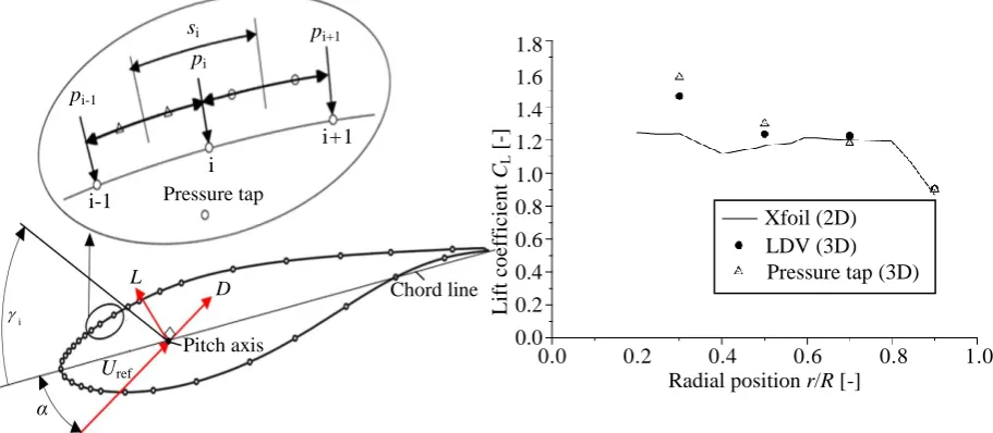
Figure 13 (a) shows the detailed variable for the sectional lift force calculation. L is the sectional lift

force that acts on the blade section perpendicular to the inflow direction (Uref). D is the sectional drag force that

acts on the blade section parallel to the inflow direction. si is the measurement taps distance between the

midpoint of the pressure measurement taps adjacent to each other in the airfoil section, γiis the tilted angle

between the i-th pressure tap and the chord line, and α is the local attack angle.

Figure 13 (b) shows estimated results of lift coefficient CL for several approach. LDV and pressure tap

measurements were performed in rotating condition while the Xfoil prediction was performed in non-rotating

condition. The lift coefficient CL is plotted against radial position r/R. In this figure, the lift coefficient CL

obtaining from LDV measurement is presented by the solid circle points the lift coefficient CL obtaining from

pressure tap measurement is presented by the triangle point. The Xfoil predicting lift coefficients from radial

position r/R = 0.2 until 0.9 are presented by the black line.

The lift coefficients from LDV and pressure tap experiments show clearly higher than Xfoil results for

inboard and mid-span regions (r/R = 0.3 and r/R = 0.5). These blade sections are contributed by the strong

complicated rotational flow to the lift enhancement. While the lift coefficients show the rare difference for the

outboard regions (r/R = 0.7 and r/R = 0.9). These blade sections are not contributed to increasing the lift

enhancement due to lowering effect of the rotation. The lift coefficients decrease rapidly from the radial position

r/R=0.8 to 0.9. It corresponds to the formation of tip vortex.

V.

CONCLUSION

This research attempted to study the velocity and pressure distributions on the rotating blade conditions. According to the wind tunnel experiments, the velocity distribution was obtained through the LDV measurement while the pressure distribution was obtained through pressure measurement taps. The following information is clarified by these measurements.

Fig. 13 (a) Sectional lift calculation from pressure taps Fig. 13 (b) Lift coefficient CL (λ = 5.2)

Pitch axis i



i-1

i

i+1

1

si

pi

pi+1

pi-1

Uref

L

D Chord line

Radial position r/R [-]

0.0 0.2 0.4 0.6 0.8 1.0 1.8

1.6

1.4

1.2

1.0

0.8

0.6

0.4

0.2

0.0

LDV (3D) Pressure tap (3D) Xfoil (2D)

L

if

t c

o

ef

ficien

t

CL

[

1. The rotational effects show obviously high influence on the inboard such as delay transition point, pressure distribution pattern changes and lift enhancement. However, the rotational effects seem to take less impact on the outboard.

2. The axial velocity component indicates that is strongly velocity gradients on the leading edge and the

trailing edge regions.

3. The tangential velocity component indicates the high positive value on the leading region due to the effect

of blade circulation.

4. The radial velocity component seems a high effect on the trailing part. However, it has a less effect to the

blade when comparing with axial and tangential velocity components.

REFERENCES

[1] GWEC. Global wind report annual market update 2014,

http://www.gwec.net/wp-content/uploads/2015/03/GWEC_Global_Wind_2014_Report_LR.pdf, Access 2015.07.25.

[2] A. Betz, Introduction to the theory of flow machines (Pergamon press, 1966).

[3] W. Rozenn, A. Ioannis, S. M. Pedersen, S. C. Michael, and H. E. Jørgensen, The influence of the wind

speed profile on wind turbine performance measurements, Wind Energy, 12(4), 2009, 348–362.

[4] G. Ronsten, Static pressure measurements on a rotating and a non-rotating 2.375 m wind turbine blade.

Comparison with 2D calculations, Journal of Wind Engineering and Industrial Aerodynamics, 39(1),

1992, 105–118.

[5] D. Wood, A three-dimensional analysis of stall-delay on a horizontal-axis wind turbine. J. WindEng. Ind.

Aerodyn.37(1), 1991, 1–14.

[6] S. Schreck, and M. Robinson, Rotational augmentation of horizontal axis wind turbine blade

aerodynamic response. Wind Energy, 5(1), 2002, 133–150.

[7] C. Sicot, P. Devinant, S. Loyer, and J. Hureau, Rotational and turbulence effects on a wind turbine blade.

Investigation of the stall mechanisms. J. Wind Eng. Ind. Aerodyn., 96(2), 2008, 1320–1331.

[8] G. G. Martínez, N. J. H. Sørensen, and Z. W. Shen, 3D Boundary Layer Study on a Rotating Wind

Turbine Blade, Journal of Physics, 37(5), 2007, 12–32.

[9] Z. Dua, and M. S. Seligb, The Effect of Rotation on the Boundary Layer of a Wind Turbine Blade,

Renewable Energy, 20(6), 2000, 167–181.

[10] T. Phengpom, Y. Kamada, T. Maeda, J. Murata, S. Nishimura, and T. Matsuno, Study on Blade Surface

Flow around Wind Turbine by Using LDV Measurements, Journal of Thermal Science, 24(2), 2015,

131139.

[11] T. Phengpom, Y. Kamada, T. Maeda, J. Murata, S. Nishimura, and T. Matsuno, Experimental

investigation of the three-dimensional flow field in the vicinity of a rotating blade, Journal of Fluid

Science and Technology, 10(2), 2015, Paper No.15-00313, 1-16.

[12] M. Drela, Xfoil 6.94 User Guide (MIT Aero & Astro Harold Youngren, 2001).

[13] L.J. Vermeer, and G.J.W. van Bussel, Velocity measurements in the near wake of a model rotor and

comparison with theoretical results, Proc. 1990 European Community Wind Energy Conference, Madrid,

Spain, 1990, 218–222.