Published online January 08, 2015 (http://www.sciencepublishinggroup.com/j/ijmea) doi: 10.11648/j.ijmea.s.2015030103.11
ISSN: 2330-023X (Print); ISSN: 2330-0248 (Online)
Coordination between traffic light system and traffic circle:
A simulation analysis approach
Ngoc-Hien Do
1, Ngoc-Quynh-Lam Le
1, Ki-Chan Nam
21Department of Industrial Systems Engineering, Faculty of Mechanical Engineering (FME), Hochiminh City University of Technology,
Hochiminh City, Vietnam
2Department of Logistics Engineering, Korea Maritime & Ocean University, Busan 606-791, the Republic of Korea
Email address:
[email protected] (Ngoc-Hien D.), [email protected] (Ngoc-Hien D.)
To cite this article:
Ngoc-Hien Do, Ngoc-Quynh-Lam Le, Ki-Chan Nam. Coordination between Traffic Light System and Traffic Circle: A Simulation Analysis Approach. International Journal of Mechanical Engineering and Applications. Special Issue: Transportation Engineering Technology. Vol. 3, No. 1-3, 2015, pp. 1-8. doi: 10.11648/j.ijmea.s.2015030103.11
Abstract:
Congestion is a serious traffic problem in many countries in the world. In road network systems, it easily arises from intersections, weak points of traffic systems. To improve their capacities, much research has been done and applied, in which traffic light and traffic circle systems are usually used. They are truly effective ones in traffic systems especially in the developing countries, where there are not much money invested for infrastructure. Whether coordination between them is better or not that is studied in this article. In addition, although many mathematic models as well as simulation programs have been used to support improving traffic problems, they are mainly used for traffic systems in developed countries and not ensure to be applicable for these in developing countries with mixed traffic conditions, Vietnam case. Therefore, a specific traffic simulation program is used. Suitable simulation models are constructed to describe as well as compare or evaluate considered alternatives including traffic light systems, traffic circle and coordination between them at the intersections. Besides, the logic of simulation models is outlined. Simulation results are, then, presented and evaluated. Finally, some conclusions are proposed.Keywords:
Traffic Simulation, Mixed Traffic Conditions, Coordination, Traffic Circle, Traffic Light System1. Introduction
Road intersection is known as where traffic flows from different directions meet, so it is considered as complex point, weak point, where accidents and congestions easily happen in traffic systems [1,2]. The complexity actually belongs to the number of roads crossed, intersection area and vehicles involved. At an intersection, many traffic controls could be used to improve traffic systems such as traffic circle, traffic light and overpass system [3,4]. Actually, the overpass system is known as the best alternative in terms of improving traffic issues, but it needs the large investment and public land available. Therefore, other alternatives are considered. Traffic circle is effective and efficient one and size of traffic circle affects directly on the entry capacity [5]. It is superior to almost every other types of traffic controls[2] and a good design to control traffic flows, so it improves intersection safety and increases the intersection’s capacity [6,7]. In the other case, traffic in a city is very much affected by traffic light controllers. An intelligent traffic light control to
minimize waiting times was suggested [8]. The optimal control frame work and treatments for different kinds of variability in traffic are used to manage conflicting requirements [9].
Because of limitations of the budget and land in cities, the overpass system is scarcely constructed. Traffic circle and traffic light system are good solutions in that case [10]. Each of them has both advantages and disadvantages, and they are usually used in individually at the intersections. Coordination between them is a suggested alternative which intends to use strong points of both alternatives [11,12,13]. The impacts of three of them are analyzed and examined under simulation analysis [14,15,16] with mixed traffic conditions.
2. Simulation Scenarios
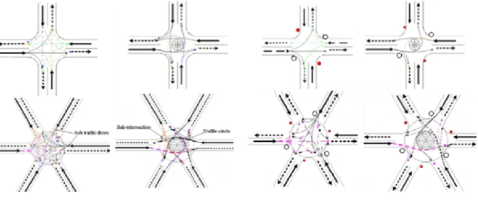
Two types of intersections were studied. The first one, 4-intersection, is a common intersection of any traffic system, which has four sub roads or where the two roads cross. Another one has more than 4 sub roads, and in this case a 6-intersection is considered as a representative, where three roads cross. Actually, when the number of sub roads at intersections increases, conflicting points increase simultaneously. Besides, if there is not any traffic control at intersections, the traffic system is so sensitive, as shown in Figure 1a. Therefore, congestion easily happens and it is not safe.
Traffic controls are applied effectively to improve traffic systems at intersections. In this research, the impacts of three alternatives were respectively considered at two intersections. Traffic circle can reduce the number of conflict points by 75% [6]. It forces vehicles travel on some traffic flows and restrict other ones as shown in Figure 1b. Another alternative usually used is traffic light systems, which can reduce 50%
of conflicting points [6] because at a period only a haft of the number of traffic flows are permitted to travel across intersections, others have to stop and wait the green signal, as shown in Figure 1c.
The other one is the suggested alternative, the coordination between traffic light system and traffic circle. Both of them are constructed and operated simultaneously at intersections. It can reduce the number of traffic flows as well as re-organize the others, as shown in Figure 1d.
Three alternatives are considered under the mixed traffic conditions, Viet Nam’s case. Their effects on intersections are evaluated on simulation analysis. A flexible simulation program developing by a group of researchers in the Industrial Systems Engineering department of Hochiminh City University of Technology in Viet Nam was used, which is mentioned detail in the next section.
Some criteria are used to evaluate alternatives. Actually, the system’s status belongs to the number of vehicles per kilometer that is defined as density factor [17]. System’s serving level or serving capacity is determined by a Volume IN factor that is the number of vehicles travelling into the system per minute. In which, the saturated points, the maximum number of vehicles that the systems could serve per minute, are found out. The system’s utility is another considering factor. It is determined based on proportions between Volume OUT factor, the number of vehicles passed the system per minute, and Volume IN factor. And the vehicles’ average speed is used to present system’s average speed. The general information flows of simulation process are shown in Figure 2.
(a)Free intersections b) Effects of traffic circle c) Effects of traffic light system d) Effects of cooperation alternative
Figure 2. The simulation process
3. A Brief Introduction of Simulation
Program
A simulation program was developed by a group of researchers of Industrial Systems Engineering department, Hochiminh City University of Technology, Vietnam. It is capable to imitate traffic behaviors under mixed traffic conditions where motorbike is the major transport in developing cities [18]. Distinct characteristics of mixed traffic system and simulation program are introduced briefly as in following paragraphs.
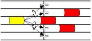
Mixed traffic system terminology is used when the traffic flow comprises both motorized and non-motorized vehicles, in which motorbike occupies a major amount. Under these conditions, vehicle can occupy any lateral position across the carriageway instead of travel on a particular lane. Besides, vehicles tend to travel in groups, in which the leader usually moves according to free flow acceleration/deceleration manners while the followers usually travel closely to their leader. In order to overtake another, cars have to change to the next lane on the left hand, while motorbikes have many choices, as shown in Figure 3. They might move one or two lanes to the left or right. It is essential to state that moving to the right side or changing more than one lane to overtake another is contrary to the law but it is the fact. Priority of lane usage is denoted from one to four, in which one means the highest priority.
Before changing lane or travelling ahead, a driver has to look for a suitable gap. When entering a traffic circle, if a driver-vehicle unit take the first exit from the traffic-circle, it usually moves toward the right. In addition, vehicles move in different velocities and accelerations/decelerations depending on drivers, vehicle physical performances, and traffic contexts. These characteristics have been imitated by many logic models.
Figure 3. Flex-passing rules of motorbike
A three-dimension coordinated system is used to model vehicles on the mixed traffic road. Vehicles are described as rectangles varying in size corresponding to their real sizes, and their locations are determined by (x, y, z) coordinates, in which (x, y) describes the location of vehicles on the same road, while z-coordinate is used when the overpass system exists. In order to best reflect the driver-vehicle unit, behaviors particularly and real world system generally, the physical, dynamic, and other relevant characteristics have been considered in the simulation program. The physical characteristics include types and sizes of vehicles, and network structure. The dynamic characteristics consist of position, velocity, acceleration, and deceleration. Turning direction, turning rate, traffic volume, and et cetera are system’s other attributes.
Travel behaviors of vehicles are modeled by using logic models. For a group of vehicles travelling on the same road, the leading vehicle movements follow acceleration/deceleration models, while movements of other vehicles are modeled by using the car-following one. Acceleration/deceleration of nth vehicle, when the gap between two vehicles is less than stipulated one, is computed by equation (1). In which, α, β, and γ are factors which are determined as shown in Table 1; Tn is the reacting time; ∆vn
is the difference in velocities between two vehicles, and Δxn
is the difference in distance between two vehicles.
= ∆ ∆ − (1)
∆ = −
∆ = −
Table 1. Coefficients
Coefficient Acceleration Deceleration
α 9.21 15.24
β -1.67 1.09
γ -0.88 1.66
This simulation program can be applied for a traffic network of a traffic node such as intersection where vehicles travel on the right. Up to six types of vehicles are simulated, which include motorbike, bicycle, car, bus, truck, and heavy truck. Actually, vehicles interact among themselves, so their parameters are updated continuously. Once an element leaves the system, output information is recorded, and system’s relative parameters are refreshed. Maximum volume, system’s average speed, etc. are recorded at each minute for each road. Velocity and travelling time of vehicles are other important information.
Some other statistical data are also recorded depending on requirements of evaluation factors. In addition, this program also provides users another utility feature to easily observe simulation process, which is animation.
4. Simulation Results and Analysis
With each intersection, alternatives are considered in respectively. At the beginning status, input data are set up at a low number of vehicles travelling into the system. It is, then, increased step by step and simulations scenarios are built and run. Outputs are recorded and analyzed. The system’s status is checked whether the system gets saturated conditions or not. When the system gets saturated conditions, the Volume IN factor get the maximum value and changes a little around and congestion easy happens. If it does not get saturated conditions, the Volume IN factor increases until the system gets saturated conditions. If congestion happened and all
alternatives were considered, simulation process is stopped. On the other hand, two procedures will be done. Data are refreshed at beginning status and another alternative is changed. The information flows are shown in Figure 4.
Figure 4. Simulation procedures
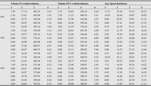
Actually, there are many types of vehicles traveling on the road; however, four of them occupy a large amount in comparison with other types. In this study, therefore, four types of vehicles are generated, which include bicycle, car, motorbike, and small truck, which are denoted from one to four, respectively as shown in Table 2. Volume IN, volume OUT, and average speed factors are recorded for each type of vehicles. Three alternatives are considered in respectively.
Table 2. Simulation results for all scenarios at two intersections
a. 4-Intersection
Volume IN (vehicle/minute) Volume OUT (vehicle/minute) Avg. Speed (km/hour)
1 2 3 4 1 2 3 4 1 2 3 4
Alt1
3.30 17.19 402.39 4.32 3.19 16.85 396.18 4.24 11.57 33.36 39.32 28.22
2.76 21.65 497.09 5.55 2.70 21.23 489.78 5.41 10.93 29.30 39.07 24.03
0.00 25.72 550.58 6.74 0.00 25.30 543.04 6.57 0.00 29.55 39.91 21.23
0.00 30.93 603.54 7.43 0.00 30.30 595.66 7.23 0.00 27.41 39.65 21.55
Alt2
3.13 16.50 385.14 4.44 3.04 16.19 378.34 4.32 8.78 24.39 31.11 24.14
3.84 21.26 476.09 5.12 3.67 20.63 467.49 4.98 9.47 21.74 30.30 18.28
0.63 24.27 555.16 6.29 0.54 23.28 544.49 6.03 5.02 19.36 29.06 16.34
0.00 25.47 578.41 6.54 0.00 23.67 563.56 6.09 0.00 18.33 28.00 16.01
0.00 26.09 604.88 6.94 0.00 23.67 587.66 6.23 0.00 15.92 27.62 13.47
0.00 27.26 605.67 6.83 0.00 24.93 589.14 6.00 0.00 16.66 27.41 13.34
0.00 26.07 600.75 6.83 0.00 23.13 584.02 5.86 0.00 14.75 27.23 12.46
Alt3
3.10 16.39 391.09 4.27 2.99 15.99 382.92 4.16 9.37 24.31 30.83 22.65
3.07 17.24 394.30 4.49 2.93 16.73 386.59 4.32 10.54 23.11 30.83 21.25
3.70 21.45 482.58 5.35 3.61 20.77 473.07 5.18 9.55 20.33 29.94 19.71
1.99 24.16 531.46 6.23 1.96 22.99 520.87 5.83 7.13 18.34 29.16 14.22
0.00 24.47 584.96 6.12 0.00 22.08 568.99 5.55 0.00 25.06 27.17 13.09
0.46 24.87 573.60 6.26 0.00 22.62 558.89 5.75 0.42 15.59 27.48 14.54
0.00 24.50 597.93 6.29 0.00 21.82 580.52 5.38 0.00 14.46 26.91 11.71
0.00 25.30 599.64 6.54 0.00 22.59 582.28 5.58 0.00 14.78 26.70 12.33
0.00 24.02 597.82 6.23 0.00 20.80 580.43 5.49 0.00 13.49 26.61 11.12
b. 6-intersection
Volume IN (vehicle/minute) Volume OUT (vehicle/minute) Avg. Speed (km/hour)
1 2 3 4 1 2 3 4 1 2 3 4
Alt1
4.33 26.00 599.76 6.60 4.11 25.51 591.45 6.40 9.27 32.70 40.04 25.96 4.86 30.04 694.32 7.70 4.44 29.48 685.43 7.51 9.74 31.40 39.96 23.93 4.36 29.29 696.25 7.65 4.22 28.30 685.54 7.40 9.30 25.31 35.38 19.31 1.24 33.38 758.70 8.53 1.21 32.77 748.01 8.28 4.95 29.11 39.74 20.61 0.33 39.23 780.65 9.63 0.33 38.37 769.63 9.36 1.76 27.15 39.98 21.49
Alt2
4.25 25.40 581.35 6.57 4.09 24.85 569.20 6.38 7.48 26.70 32.34 22.74 4.36 29.07 686.95 7.65 3.89 28.21 672.70 7.40 8.62 24.25 31.54 19.70 4.64 29.93 697.52 7.37 4.22 29.21 682.50 7.15 8.76 24.66 31.42 22.66 4.91 30.75 690.48 7.65 4.69 29.93 675.68 7.37 8.01 24.66 31.63 20.69
Alt3
4.28 24.85 574.81 6.63 4.06 24.15 561.67 6.49 7.34 23.23 31.58 18.45 4.72 27.55 695.56 7.18 4.44 26.12 680.38 6.79 8.39 20.36 30.84 17.74 4.72 28.68 674.77 7.54 4.55 27.74 659.45 7.26 8.02 21.37 30.98 18.19 1.88 33.16 743.04 8.28 1.88 32.05 725.90 7.95 5.85 19.07 30.26 14.49 0.33 36.91 764.19 9.55 0.33 35.53 746.63 9.16 1.67 18.91 30.02 16.76 0.22 36.61 758.86 9.66 0.22 35.20 741.03 9.36 1.20 19.46 30.36 17.18 0.22 37.96 768.97 9.83 0.22 36.39 749.97 9.39 1.67 18.09 29.83 14.35 0.00 37.63 767.39 9.72 0.00 36.08 750.03 9.22 0.00 18.43 29.43 14.60 0.75 36.69 755.61 9.72 0.75 34.67 733.60 9.06 2.96 15.95 26.53 14.07
Alt1: Traffic circle, Alt2: Traffic light system, Alt3: Coordination
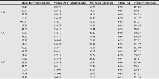
To be easier to analyze, the simulation results are converted into car’s indexes usually used in homogeneous traffic systems of developing countries. The vehicle conversion rate system, which resulted from another research [19] is applied, see Appendix 1. The converted results are then presented as shown in Table 3 for both intersections, where the Volume IN and Volume OUT factors present the
number of cars travelling into and leaving out the system per minute in respectively, Average Speed factor presents cars’ average speed when they travel across the system, Utility factor presents the ratios between the number of vehicle serving by the system and travelling into the system, and Density factor presents its busy level.
Table 3. Converted simulation results.
4-Intersection
Volume IN (vehicle/minute) Volume OUT (vehicle/minute) Avg. Speed (km/hour) Utility (%) Density (vehicle/km)
Alt1
103.47 101.75 38.76 0.98 157.52
127.77 125.72 38.37 0.98 196.6
142.28 140.17 39.24 0.99 214.33
158.73 156.33 38.86 0.98 241.39
Alt2
99.38 97.55 30.60 0.98 191.31
123.32 120.75 29.67 0.98 244.19
141.61 138.18 28.51 0.98 290.8
147.37 142.16 27.49 0.98 310.27
153.67 147.11 27.03 0.96 326.56
152.71 145.47 26.62 0.95 327.92
154.89 148.43 26.84 0.96 331.79
Alt3
100.27 98.07 30.33 0.98 193.99
101.97 99.68 30.27 0.98 197.58
124.97 122.17 29.29 0.98 250.27
137.42 133.73 28.47 0.97 281.81
145.76 139.84 26.90 0.96 311.96
147.25 141.11 26.59 0.96 318.41
150.04 142.98 26.33 0.95 325.84
149.48 142.06 26.02 0.95 327.57
151.43 144.30 26.13 0.95 331.38
6-Intersection
Volume IN (vehicle/minute) Volume OUT (vehicle/minute) Avg. Speed (km/hour) Utility (%) Density (vehicle/km)
Alt1
154.88 152.40 39.40 0.98 232.1
179.20 176.42 39.26 0.98 269.6
193.99 190.98 39.05 0.98 293.48
197.05 193.90 38.75 0.98 300.25
204.76 201.43 39.15 0.98 308.70
Alt2
150.52 147.25 31.84 0.98 277.50
176.40 172.17 31.08 0.98 332.39
179.12 174.94 31.07 0.98 337.80
179.26 175.07 30.93 0.98 339.63
Alt3
148.74 145.15 30.93 0.98 281.54
173.69 169.32 30.32 0.97 335.11
176.35 171.33 30.20 0.97 340.44
190.78 185.93 29.57 0.97 377.27
197.75 192.48 29.71 0.97 388.77
199.08 193.81 29.36 0.97 396.12
201.29 195.48 29.10 0.97 403.02
200.39 194.89 28.76 0.97 406.59
197.56 190.50 25.89 0.96 441.47
Alt1: Traffic circle, Alt2: Traffic light system, Alt3: Coordination
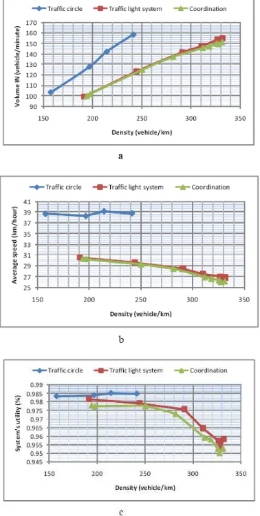
Figure 5. Comparisons among alternatives on system’s serving level, average speed and utility for the 4-intersection.
The impacts of alternatives are different because they depend on types of intersections and on the Density factor,
the system’s busy level. With the 4-intersection, there are two stages of the system depending on Density factor’s value. When it is less than 242, the traffic circle alternative is the best one in comparisons with other ones. However, it could not serve or congestion happened when the Density factor got more than 242 vehicles per kilometer, while other ones could serve, as shown in Figure 5. And the traffic light system alternative got a little bit better than the coordination one.
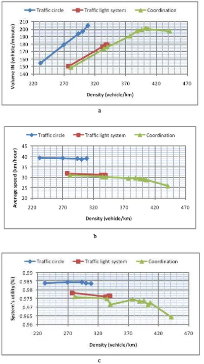
With the 6-intersection, there are three stages of the system that depends on the Density factor. If it is less than 308, the best alternative is, similarly with previous one, the traffic circle alternative. On the other hand, when the Density factor gets more than 339 cars per kilometer, the system becomes so busy and only the coordination alternative could serve the system, while congestion happens in other ones. The other system’s stage is when the Density factor gets from 308 to 339 cars per kilometer. Congestion happens with the traffic circle alternative and traffic light system one gets a little bit better than the coordination alternative, as shown in Figure 6. When making comparisons in separately for each criterion, with the system’s serving level, the traffic circle alternative reaches the maximum values in both intersections. However, with the 4-intersection, the maximum values of Volume IN factor of all alternatives are 158, 154 and 151 in respectively, nearly equal as shown in Figure 5a. With the 6-intersection, the coordination alternative gets the second place and a little bit lower than the best one, 201 in comparison with 204, but impressively higher than that’s value, 179, of the traffic light system alternative, as shown in Figure 6a.
as shown in Figure 5b and 6b.
Figure 6. Comparisons among alternatives on system’s serving level, average speed and utility for the 6-intersection.
With system’s utility factor, although the coordination alternative gets the lowest value, it is actually too high because the simulation results are reported when congestion did not happen, as shown in Figure 5c and 6c.
The summarized results are shown in Table 4. Determining
which alternative should be used belongs to the system’s status or density factor. In general, when the system is not so busy, the traffic circle should be used to control traffic flows. In the other hand, the coordination alternative is so useful.
5. Conclusions
In this study, based on simulation analysis, the impacts and effects of traffic controls including traffic circle, traffic light system and coordination alternative were considered on two common intersections. They are studied under the mixed traffic conditions. The study shows that the coordination alternative should be used to control traffic flows at intersections. Both of the traffic circle and traffic light system should be constructed. Depending on the density of vehicles on the roads of system’s busy level, the traffic light system whether operates or not, as shown in Figure 7. It operates that means the coordination alternative fully affects the system. In another case, traffic flows is only affected by the traffic circle. The strong points of both traffic controls are used.
Figure 7. Alternatives to use the traffic light system
However, this study only focus on suggesting alternatives to improve traffic systems in mixed traffic conditions where resources such as budget and public land are limited. Actually, the other better alternatives such as overpass system could be used if required conditions are met.
Table 4. Summarized results
4-intersection
Factors Capacity Average speed Utility
Density < 250 [250, 330) < 250 [250, 330) < 250 [250, 330)
Traffic circle Very good X Very good X Very good X Traffic light system Good Very good Good Good Good Very good Coordination Good Good Good Good Good Good
6-intersection
Factors Capacity Average speed Utility
Density < 250 (290, 330) [330, 440) < 250 (250, 330) [330, 440) < 250 (250, 330) [330, 440) Traffic circle Very good X X Very good X X Very good X X Traffic light system Good Very good X Good Very good X Good Good X Coordination Good Good Very good Good Good Very good Good Good Good
Appendixes
Appendix 1. Vehicle converted coefficients
Bicycle Car Motorbike Small truck Coeff. 1.6295 1 5.014 1
References
[1] Lord D., Schalkwyk I.V., Chrysler S., and Staplin L. (2007), A strategy to reduce older driver injuries at intersections using more accommodating roundabout design practices, Accident Analysis and Prevention, 39, 427-432.Brabander B.D. and Vereeck L. (2007) Safety effects of roundabouts in Flanders: Signal type, speed limits and vulnerable road users, Accident Analysis and Prevention, ELSEVIER, 39, 591-599.
[2] Russell E.R., Lutrell, and Rys M. (2002), Roundabout studies in Kansas, a presentation at 4th Transportation Specialty Conference of Canadian Society for Civil Engineering, Montreal, Quebec, Canada, 5-8 June 2002.
[3] Hashim M.N. A. (2003), Dynamic vehicular delay comparison between a police-controlled roundabout and a traffic signal, Transportation Research Part A, PERGAMON, 37, 681-688.
[4] Herty M., Klar A., and. Singh A. K (2006), An ODE traffic network model, Journal of Computational and Applied Mathematics, Elsevier, 203, 419-436.Heydecker (2004).
[5] Hossain M. (1999), Capacity estimation of traffic circles under mixed traffic conditions using micro-simulation technique, Transportation Research Part A, PERGAMON, 33, 47-61.
[6] Stamatiadis N. and Kirk A. (2005), Modern roundabouts: a guide for applications, Community Transportation Innovation Academy, Kentucky.
[7] Tove H. and Ivanka O.B (2007), The effect of roundabout design features on cyclic accident rate, Accident Analysis and Prevention, ELSEVIER, 39, 300-307.
[8] Marco Wiering, Intelligent Traffic Light Control, April 2003. http://www.ercim.org/publication/Ercim_News/enw53/wierin g.html
[9] Heydecker (2004), Objectives, stimulus and feedback in signal control of road traffic, IST Journal, Vol.8, 63-76.
[10] Coelho M.C., Farias T.L., and Rouphail N.M (2006), Effect of roundabout operations on pollutant emissions, Transportation part D, ELSEVIER, 11, 333-343.
[11] Huang D.W. (2007), Phase diagram of a traffic roundabout, Physical A, Science Direct, 383, 603-612.
[12] Elvik R. (2003), Effects on road safety of converting intersections to roundabouts: review of evidence from non-U.S. studies, Transportation Research Board, 1847.
[13] Elvik R. and Vaa T. (2004), The handbook of Road safety measures, Elsevier, 1078pp.
[14] Kelton W.D., Sadowski R.P., and Sadowski D.A. (1998), Simulation with Arena, USA: McGraw-Hill.
[15] Law A.M. and Kelton W.D. (1999), Simulation Modeling and Analysis, Singapore: McGraw-Hill.
[16] Takahashi M., Nakanishi T., Miyoshi I., and Fujikura T. (2002), An evaluation of the road traffic system simulator PIMTRACS by PIM, Mathematics and Computers in Simulation, Elsevier, 59, pp. 45-56
[17] Gazis D.C (2002), Traffic theory, New York, Boston, Dordrecht, London, Moscow: Kluwer Academic Publishers.
[18] Le N.Q.L., Do N.H., Kim T.W., and Nam K.C (2008), Special traffic problems in Vietnam: Simulation method, the Modeling, Simulation & Gaming Student Capstone Conference 2008, Virginia, U.S.A, April 10, 2008, and being revised to publish at International Journal of Simulation and process modeling, Inderscience.
[19] Do N.H, Le N.Q.L, and Nam K.C. (2008), Conversion rate from motorbike to car: Simulation analysis, Proceedings 24th European Conference on Modelling and Simulation.
Biography
Ngoc-Hien Do is a lecturer of Department of Industrial Systems Engineering (ISE), Hochiminh City University of Technology (HCMUT), Vietnam. He received BEng in Mechanical Engineering from HCMUT, Master of Science and PhD in Logistics Department from Korea Maritime University (KMU), the Republic of Korea.
Quynh-Lam Ngoc-Le is a lecturer of Department of Industrial Systems Engineering, Hochiminh City University of Technology (HCMUT), Vietnam. She received BEng in Electronics Engineering from HCMUT, MEng in Industrial Systems Engineering, Thailand, and PhD in Logistics Department from Korea Maritime University (KMU), the Republic of Korea.