Journal of Machine Learning Research, 7:793–815, 2006.
Learning Image Components for Object Recognition
M. W. Spratling
Division of Engineering, King’s College London. UK.
and Centre for Brain and Cognitive Development, Birkbeck College, London. UK.
Abstract
In order to perform object recognition it is necessary to learn representations of the underlying components of images. Such components correspond to objects, object-parts, or features. Non-negative matrix factorisation is a generative model that has been specifically proposed for finding such meaningful representations of image data, through the use of non-negativity constraints on the factors. This article reports on an empirical investigation of the performance of non-negative matrix factorisation algorithms. It is found that such algorithms need to impose additional constraints on the sparseness of the factors in order to successfully deal with occlusion. However, these constraints can themselves result in these algorithms failing to identify image components under certain conditions. In contrast, a recognition model (a competitive learning neural network algorithm) reliably and accurately learns representations of elementary image features without such constraints.
Keywords: non-negative matrix factorisation; competitive learning; dendritic inhibition; object recognition
1
Introduction
An image usually contains a number of different objects, parts, or features and these components can occur in dif-ferent configurations to form many distinct images. Identifying the underlying components which are combined to form images is thus essential for learning the perceptual representations necessary for performing object recog-nition. Non-negative matrix factorisation (NMF) has been proposed as a method for finding such parts-based decompositions of images (Lee and Seung,1999;Feng et al.,2002;Liu et al.,2003;Liu and Zheng,2004; Li et al.,2001;Hoyer,2002,2004). However, the performance of this method has not been rigorously or quantita-tively tested. Instead, only a subjective assessment has been made of the quality of the components that are learnt when this method is applied to processing images of, for example, faces (Lee and Seung,1999;Hoyer,2004;Li et al.,2001;Feng et al.,2002). This paper thus aims to quantitatively test, using several variations of a simple standard test problem, the accuracy with which NMF identifies elementary image features. Furthermore, non-negative matrix factorisation assumes that images are composed of a linear combination of features. However, in reality the superposition of objects or object parts does not always result in a linear combination of sources but, due to occlusion, results in a non-linear combination. This paper thus also aims to investigate, empirically, how NMF performs when tested in more realistic environments where occlusion takes place. Since competitive learn-ing algorithms have previously been applied to this test problem, and neural networks are a standard technique for learning object representations, the performance of NMF is compared to that of an unsupervised neural network learning algorithm applied to the same set of tasks.
2
Method
2.1
Non-Negative Matrix Factorisation
Given anmbypmatrixX= [~x1, . . . , ~xp], each column of which contains the pixel values of an image (i.e.,Xis
a set of training images), the aim is to find the factorsAandYsuch that:
X≈AY
WhereAis anmbynmatrix the columns of which contain basis vectors, or components, into which the images can be decomposed, andY= [~y1, . . . , ~yp]is annbypmatrix containing the activations of each component (i.e.,
the strength of each basis vector in the corresponding training image). A training image (~xk) can therefore be
reconstructed as a linear combination of the image components contained inA, such that~xk ≈A~yk.
Acronym Description Reference
Non-ne
g
ati
v
e
Matrix
F
actorisa
tion
Algorithms
nmfdiv NMF with divergence objective (Lee and Seung,2001)
nmfmse NMF with euclidean objective (Lee and Seung,2001)
lnmf Local NMF (Li et al.,2001;Feng et al.,
2002)
snmf Sparse NMF (α= 1) (Liu et al.,2003)
nnsc Non-negative sparse coding (λ= 1) (Hoyer,2002)
nmfsc (A) NMF with a sparseness constraint of 0.5 on the
ba-sis vectors
(Hoyer,2004)
nmfsc (Y) NMF with a sparseness constraint of 0.7 on the
ac-tivations
(Hoyer,2004)
nmfsc (A&Y) NMF with sparseness constraints of 0.5 on the
ba-sis vectors and 0.7 on the activations
(Hoyer,2004)
Neural Netw
ork
Algorithms
nndi Dendritic inhibition neural network with non-negative weights
di Dendritic inhibition neural network (Spratling and Johnson,
2002,2003)
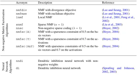
Table 1: The algorithms tested in this article. These include a number of different algorithms for finding
matrix factorisations under non-negativity constraints and a neural network algorithm for performing competitive learning through dendritic inhibition.
to be mutually orthogonal, and independent components analysis (ICA) constrains the rows ofYto be statistically independent. Non-negative matrix factorisation is a method that seeks to find factors (of a non-negative matrix X) under the constraint that bothAandYcontain only elements with non-negative values. It has been proposed that this method is particularly suitable for finding the components of images, since from the physical properties of image formation it is known that image components are non-negative and that these components are combined additively (i.e., are not subtracted) in order to generate images. Several different algorithms have been proposed for finding the factorsAandYunder non-negativity constraints. Those tested here are listed in Table1.
Algorithmsnmfdivandnmfmseimpose non-negativity constraints solely, and differ only in the objective function that is minimised in order to find the factors. All the other algorithms extend non-negative matrix fac-torisation by imposing additional constraints on the factors. Algorithmlnmfimposes constraints that require the columns ofAto contain as many non-zero elements as possible, andYto contain as many zero elements as possible. This algorithm also requires that basis vectors be orthogonal. Both algorithmssnmfandnnscimpose constraints on the sparseness ofY. Algorithmnmfscallows optional constraints to be imposed on the sparseness of either the basis vectors, the activations, or both. This algorithm was used with three combinations of sparseness constraints. Fornmfsc (A)a constraint on the sparseness of the basis vectors was applied. This constraint re-quired that each column ofAhad a sparseness of 0.5. Valid values for the parameter controlling sparseness could range from 0 (which would produce completely distributed basis vectors) to a value of 1 (which would produce completely sparse basis vectors). Fornmfsc (Y)a constraint on the sparseness of the activations was applied. This constraint required that each row ofY had a sparseness of 0.7 (where sparseness is in the range[0,1], as for the constraint onA). Fornmfsc (A&Y)these same constraints were imposed on both the sparseness of ba-sis vectors and the activations. For thenmfscalgorithm, fixed values for the parameters controlling sparseness were used in order to provide a fairer comparison with the other algorithms all of which used constant parameter settings. Furthermore, since all the test cases studied are very similar, it is reasonable to expect an algorithm to work across them all without having to be tuned specifically to each individual task. The particular parameter values used were selected so as to provide the best overall results across all the tasks. The effect of changing the sparseness parameters is described in the discussion section.
2.2
Dendritic Inhibition Neural Network
Weights
Feedback
1k 2k
1k 2k 3k
11
X
Y
Y
X
X
A
(a) Feedforward Weights 1k 2k1k 2k 3k
11
X
Y
Y
X
X
W
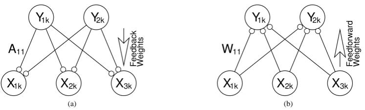
(b)Figure 1: (a) A generative neural network model: feedback connections enable neural activations (~yk)
to reconstruct an input pattern (~xk). (b) A recognition neural network model: feedforward connections
cause neural activations (~yk) to be generated in response to an input pattern (~xk). Nodes are shown as
large circles and excitatory synapses as small open circles.
synaptic weightsA(see Figure1a). In contrast, traditional neural network algorithms have attempted to learn a set of feedforward (recognition) weightsW(see Figure1b), such that:
Y= f (W,X)
WhereWis annbymmatrix of synaptic weight values,X= [x~1, . . . , ~xp]is anmbypmatrix of training images,
andY= [~y1, . . . , ~yp]is annbypmatrix containing the activation of each node in response to the corresponding
image. Typically, the rows ofWform templates that match image features, so that individual nodes become active in repose to the presence of specific components of the image. Nodes thus act as ‘feature detectors’ (Barlow,1990,
1995).
Many different functions are possible for calculating neural activations and many different learning rules can be defined for finding the values of W. For example, algorithms have been proposed for performing vector quantization (Kohonen,1997;Ahalt et al.,1990), principal components analysis (Oja,1992;Fyfe,1997b;F¨oldi´ak,
1989), and independent components analysis (Jutten and Herault,1991;Charles and Fyfe,1997; Fyfe,1997a). Many of these algorithms impose non-negativity constraints on the elements ofYandWfor reasons of biological plausibility, since neural firing rates are positive and since synapses can not change between being excitatory and being inhibitory. In general, such algorithms employ different forms of competitive learning, in which nodes compete to be active in response to each input pattern. Such competition can be implemented using a number of different forms of lateral inhibition. In this paper, a competitive learning algorithm in which nodes can inhibit the inputs to other nodes is used. This form of inhibition has been termed dendritic inhibition or pre-integration lateral inhibition. The full dendritic inhibition model (Spratling and Johnson,2002,2003) allows negative synaptic weight values. However, in order to make a fairer comparison with NMF, a version of the dendritic inhibition algorithm in which all synaptic weights are restricted to be non-negative (by clipping the weights at zero) is also used in the experiments described here. The full model will be referred to by the acronymdiwhile the non-negative version will be referred to asnndi(see Table1).
In a neural network model, an input image (~xk) generates activity (~yk) in the nodes of a neural network such
that~yk = f (W, ~xk). In the dendritic inhibition model, the activation of each individual node is calculated as:
yjk=W~x0kj
where~x0kjis an inhibited version of the input activations (~xk) that can differ for each node. The values of~x0kjare
calculated as:
x0ikj=xik
1−α
n max
r=1 (r6=j)
(
wri maxm
q=1{wrq}
yrk maxn
q=1{yqk}
)
+
.
Whereαis a scale factor controlling the strength of lateral inhibition, and(v)+is the positive half-rectified value ofv. The steady-state values ofyjkwere found by iteratively applying the above two equations, increasing the
value ofαfrom 0 to 6 in steps of 0.25, while keeping the input image fixed.
inhibit other nodes from responding to that feature. On the other hand, if an active node receives a weak weight from a feature then it will only weakly inhibit other nodes from responding to that feature. In this manner, each node can selectively ‘block’ its preferred inputs from activating other nodes, but does not inhibit other nodes from responding to distinct stimuli.
All weight values were initialised to random values chosen from a Gaussian distribution with a mean of 1
m
and a standard deviation of0.001mn. This small degree of noise on the initial weight values was sufficient to cause bifurcation of the activity values, and thus to cause differentiation of the receptive fields of different nodes through activity-dependent learning. Previous results with this algorithm have been produced using noise (with a similarly small magnitude) applied to the node activation values. Using noise applied to the node activations, rather than the weights, produces similar results to those reported in this article. However, noise was only applied to the initial weight values, and not to the node activations, here to provide a fairer comparison to the deterministic NMF algorithms. Note that a node which still has its initial weight values (i.e., a node which has not had its weights modified by learning) is described as ‘uncommitted’.
Synaptic weights were adjusted using the following learning rule (applied to weights with values greater than or equal to zero):
∆wji=
(xik−¯xk)
Pm
p=1xpk
(yjk−y¯k)
+
(1)
Wherex¯kis the mean value of the pixels in the training image (i.e.,x¯k =m1 P m
i=1xik), andy¯kis the mean of the
output activations (i.e.,y¯k = n1P n
j=1yjk). Following learning, synaptic weights were clipped at zero such that
wji= (wji)
+
and were normalised such thatPm
i=1(wji)
+
≤1.
This learning rule encourages each node to learn weights selective for a set of coactive inputs. This is achieved since when a node is more active than average it increases its synaptic weights to active inputs and decreases its weights to inactive inputs. Hence, only sets of inputs which are consistently coactive will generate strong afferent weights. In addition, the learning rule is designed to ensure that different nodes can represent stimuli which share input features in common (i.e., to allow the network to represent overlapping patterns). This is achieved by rectifying the post-synaptic term of the rule so that no weight changes occur when the node is less active than average. If learning was not restricted in this way, whenever a pattern was presented all nodes which represented patterns with overlapping features would reduce their weights to these features.
For the algorithmdi, but not for algorithmnndi, the following learning rule was applied to weights with values less than or equal to zero:
∆wji=
x0ikj−0.5xik
−
Pn
p=1ypk
(yjk−y¯k) (2)
Where(v)−is the negative half-rectified value ofv. Negative weights were clipped at zero such thatw
ji= (wji)
−
and were normalised such thatPm
i=1(wji)
−
≥ −1. Note that for programming convenience a single synapse is allowed to take either excitatory or inhibitory weight values. In a more biologically plausible implementation two separate sets of afferent connections could be used: the excitatory ones being trained using equation1and the inhibitory ones being trained using a rule similar to equation2.
The negative weight learning rule has a different form from the positive weight learning rule as it serves a different purpose. The negative weights are used to ensure that each image component is represented by a distinct node rather than by the partial activation of multiple nodes each of which represents an overlapping image component. A full explanation of this learning rule is provided together with a concrete example of its function in section3.3.
3
Results
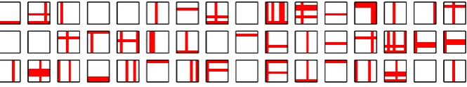
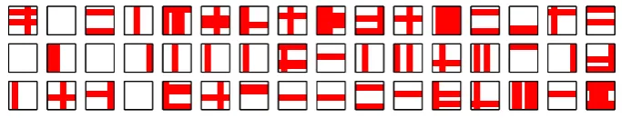
Figure 2: Typical training patterns for the standard bars problem. Horizontal and vertical bars in 8x8
pixel images are independently selected to be present with a probability of18. Dark pixels indicate active inputs.
epochs, while the neural network algorithms were trained for at most 100 epochs (since the value ofpwas 100 or greater).
3.1
Standard Bars Problem
The bars problem (and its variations) is a benchmark task for the learning of independent image features (F¨oldi´ak,
1990;Saund,1995;Dayan and Zemel,1995;Hinton et al.,1995;Harpur and Prager,1996;Hinton and Ghahra-mani,1997;Frey et al.,1997;Fyfe,1997b;Charles and Fyfe,1998;Hochreiter and Schmidhuber,1999;Meila and Jordan,2000;Plumbley,2001;O’Reilly,2001;Ge and Iwata,2002;L¨ucke and von der Malsburg,2004). In the standard version of the bars problem, as defined byF¨oldi´ak(1990), training data consists of 8 by 8 pixel images in which each of the 16 possible (one-pixel wide) horizontal and vertical bars can be present with a probability of
1
8. Typical examples of training images are shown in Figure2.
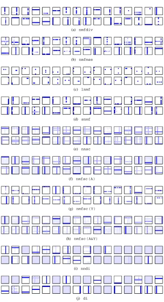
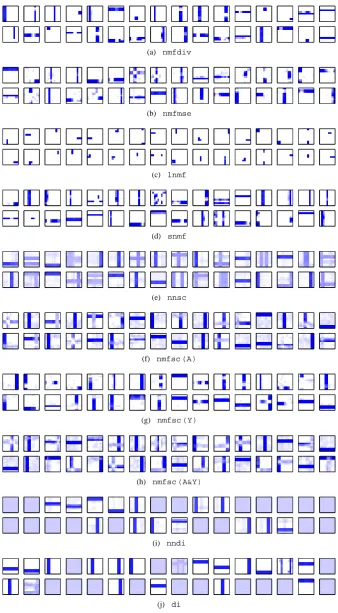
In the first experiment the algorithms were trained on the standard bars problem. Twenty-five trials were performed withp= 100, and, withp= 400. The number of components that each algorithm could learn (n) was set to 32. Typical examples of the (generative) weights learnt by each NMF algorithm (i.e., the columns of Areshaped as 8 by 8 pixel images) and of the (recognition) weights learnt by the neural network algorithms (i.e., the rows ofWreshaped as 8 by 8 pixel images) are shown in Figure3. It can be seen that the NMF algorithms tend to learn a redundant representation, since the same bar can be represented multiple times. In contrast, the neural network algorithms learnt a much more compact code, with each bar being represented by a single node. It can also be seen that many of the NMF algorithms learnt representations of bars in which pixels were missing. Hence, these algorithms learnt random pieces of image components rather than the image components themselves. In contrast, the neural network algorithms (and algorithmsnnsc, nmfsc (A), andnmfsc (A&Y)) learnt to represent complete image components.
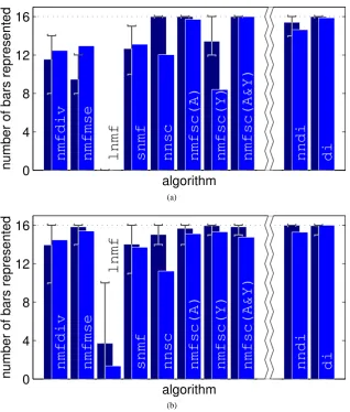
To quantify the results, the following procedure was used to determine the number of bars represented by each algorithm in each trial. For each node, the sum of the weights corresponding to each row and column of the input image was calculated. A node was considered to represent a particular bar if the total weight corresponding to that bar was twice that of the sum of the weights for any other row or column and if the minimum weight in the row or column corresponding to that bar was greater than the mean of all the (positive) weights for that node. The number of unique bars represented by at least one basis vector, or one node of the network, was calculated, and this value was averaged over the 25 trials. The mean number of bars (i.e., image components) represented by each algorithm is shown in Figure4a. Good performance requires both accuracy (finding all the image components) and reliability (doing so across all trials). Hence, the average number of bars represented needs to be close to 16 for an algorithm to be considered to have performed well. It can be seen that whenp= 100, most of the NMF algorithms performed poorly on this task. However, algorithmsnmfsc (A)andnmfsc (A&Y)produced good results, representing an average of 15.7 and 16 components respectively. This compares favourably to the neural network algorithms, withnndirepresenting 14.6 anddirepresenting 15.9 of the 16 bars. When the number of images in the training set was increased to 400 this improved the performance of certain NMF algorithms, but lead to worse performance in others. Forp= 400, every image component in every trial was found by algorithms
nnsc,nmfsc (A),nmfsc (A&Y)anddi.
(a) nmfdiv
(b) nmfmse
(c) lnmf
(d) snmf
(e) nnsc
(f) nmfsc (A)
(g) nmfsc (Y)
(h) nmfsc (A&Y)
(i) nndi
(j) di
Figure 3: Typical generative or recognition weights learnt by 32 basis vectors or nodes when each
0
4
8
12
16
number of bars represented
nmfdiv
nmfmse
lnmf
snmf
nnsc
nmfsc(A)
nmfsc(Y)
nmfsc(A&Y)
nndi
di
algorithm
(a)
0
4
8
12
16
number of bars represented
nmfdiv
nmfmse
lnmf
snmf
nnsc
nmfsc(A)
nmfsc(Y)
nmfsc(A&Y)
nndi
di
algorithm
(b)
Figure 4: Performance of each algorithm when trained on the standard bars problem. For (a) 32, and
(b) 16 basis vectors or nodes. Each bar shows the mean number of components correctly identified by each algorithm when tested over 25 trials. Results for different training set sizes are shown: the lighter, foreground, bars show results forp= 100, and the darker, background, bars show results forp= 400. Error bars show best and worst performance, across the 25 trials, whenp= 400.
image components with an excess of nodes. Across both these experiment thediversion of the neural network algorithm performs as well as or better than any of the NMF algorithms.
3.2
Bars Problems Without Occlusion
To determine the effect of occlusion on the performance of each algorithm further experiments were performed using versions of the bars problem in which no occlusion occurs. Firstly, a linear version of the standard bars problem was used. Similar tasks have been used by Plumbley (2001) and Hoyer (2002). In this task, pixel values are combined additively at points of overlap between horizontal and vertical bars. As with the standard bars problem, training data consisted of 8 by 8 pixel images in which each of the 16 possible (one-pixel wide) horizontal and vertical bars could be present with a probability of18. All the algorithms were trained withp= 100
and withp= 400using 32 nodes or basis vectors. The number of unique bars represented by at least one basis vector, or one node of the network, was calculated, and this value was averaged over 25 trials. The mean number of bars represented by each algorithm is shown in Figure5a.
Another version of the bars problem in which occlusion is avoided is one in which horizontal and vertical bars do not co-occur. Similar tasks have been used byHinton et al.(1995);Dayan and Zemel(1995);Frey et al.
0
4
8
12
16
number of bars represented
nmfdiv
nmfmse
lnmf
snmf
nnsc
nmfsc(A)
nmfsc(Y)
nmfsc(A&Y)
nndi
di
algorithm
(a)
0
4
8
12
16
number of bars represented
nmfdiv
nmfmse
lnmf
snmf
nnsc
nmfsc(A)
nmfsc(Y)
nmfsc(A&Y)
nndi
di
algorithm
(b)
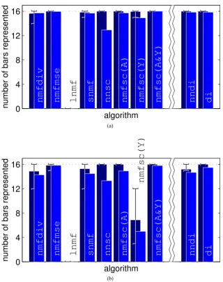
Figure 5: Performance of each algorithm when trained on (a) the linear bars problem, and (b) the
one-orientation bars problem, with 32 basis vectors or nodes. Each bar shows the mean number of components correctly identified by each algorithm when tested over 25 trials. Results for different training set sizes are shown: the lighter, foreground, bars show results forp= 100, and the darker, background, bars show results forp= 400. Error bars show best and worst performance, across the 25 trials, whenp= 400.
withp= 100and withp= 400using 32 nodes or basis vectors. The number of unique bars represented by at least one basis vector, or one node of the network, was calculated, and this value was averaged over 25 trials. The mean number of bars represented by each algorithm is shown in Figure5b.
For both experiments using training images in which occlusion does not occur, the performance of most of the NMF algorithms is improved considerably in comparison to the standard bars problem. The neural network algorithms also reliably learn the image components as with the standard bars problem.
3.3
Bars Problem With More Occlusion
To further explore the effects of occlusion on the learning of image components a version of the bars problem with double-width bars was used. Training data consisted of 9 by 9 pixel images in which each of the 16 possible (two-pixel wide) horizontal and vertical bars could be present with a probability18. The image size was increased by one pixel to keep the number of image components equal to 16 (as in the previous experiments). In this task, as in the standard bars problem, perpendicular bars overlap; however, the proportion of overlap is increased. Furthermore, neighbouring parallel bars also overlap (by 50%). Typical examples of training images are shown in Figure6.
Figure 6: Typical training patterns for the double-width bars problem. Two pixel wide horizontal and
vertical bars in a 9x9 pixel image are independently selected to be present with a probability of18. Dark pixels indicate active inputs.
each algorithm could learn (n) was set to 32. Typical examples of the (generative) weights learnt by each NMF algorithm and of the (recognition) weights learnt by the neural network algorithms are shown in Figure7. It can be seen that the majority of the NMF algorithms learnt redundant encodings in which the basis vectors represent parts of image components rather than complete components. In contrast, the neural network algorithms (and the
nnscalgorithm) learnt to represent complete image components.
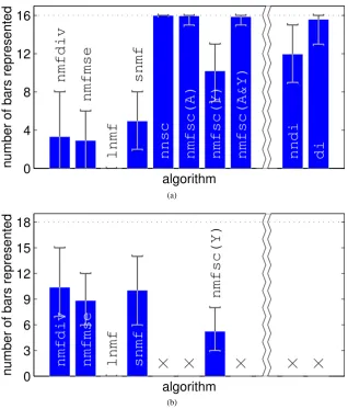
The following procedure was used to determine the number of bars represented by each algorithm in each trial. For each node, the sum of the weights corresponding to every double-width bar was calculated. A node was considered to represent a particular bar if the total weight corresponding to that bar was 1.5 times that of the sum of the weights for any other bar and if the minimum weight of any pixel forming part of that bar was greater than the mean of all the (positive) weights for that node. The number of unique bars represented by at least one basis vector, or one node of the network, was calculated. The mean number of two-pixel-wide bars, over the 25 trials, represented by each algorithm is shown in Figure8a. This set of training images could be validly, but less efficiently, represented by 18 one-pixel-wide bars. Hence, the mean number of one-pixel-wide bars, represented by each algorithm was also calculated and this data is shown in Figure8b. The number of one-pixel-wide bars represented was calculated using the same procedure used to analyse the previous results (as stated in section3.1). It can be seen that the majority of the NMF algorithms perform very poorly on this task. Most fail to reliably represent either double- or single-width bars. However, algorithmsnnsc,nmfsc (A)andnmfsc (A&Y)do succeed in learning the image components. The dendritic inhibition algorithm, with negative weights, also suc-ceeds in identifying all the double-width bars in most trials. However, the non-negative version of this algorithm performs less well. This result illustrates the need to allow negative weight values in this algorithm in order to robustly learn image components. Negative weights are needed to disambiguate a real image component from the simultaneous presentation of partial components. For example, consider part of the neural network that is receiv-ing input from four pixels that are part of four separate, neighbourreceiv-ing, columns of the input image (as illustrated in Figure9). Assume that two nodes in the output layer (nodes1and3) have learnt weights that are selective to two neighbouring, but non-overlapping, double-width bars (bars1and3). When the double-width bar (bar2) that overlaps these two represented bars is presented to the input, then the network will respond by partially activating nodes1and3. Such a representation is reasonable since this input pattern could be the result of the co-activation of partially occluded versions of the two represented bars. However, if bar2recurs frequently then it is unlikely to be caused by the chance co-occurrence of multiple, partially occluded patterns, and is more likely to be an independent image component that should be represented in a similar way to the other components (i.e., by the activation of a specific node tuned to that feature). One way to ensure that in such situations the network learns all image components is to employ negative synaptic weights. These negative weights are generated when a node is active and inputs, which are not part of the nodes’ preferred input pattern, are inhibited. This can only occur when multiple nodes are co-active. If the pattern, to which this set of co-active nodes are responding, re-occurs then the negative weights will grow. When the negative weights are sufficiently large the response of these nodes to this particular pattern will be inhibited, enabling an uncommitted node to successfully compete to represent this pattern. On the other hand, if the pattern, to which this set of co-active nodes are responding, is just due to the co-activation of independent input patterns then the weights will return toward zero on subsequent presentations of these patterns in isolation.
3.4
Bars Problem with Unequal Components
(a) nmfdiv
(b) nmfmse
(c) lnmf
(d) snmf
(e) nnsc
(f) nmfsc (A)
(g) nmfsc (Y)
(h) nmfsc (A&Y)
(i) nndi
(j) di
Figure 7: Typical generative or recognition weights learnt by 32 basis vectors or nodes when each
0
4
8
12
16
number of bars represented
nmfdiv
nmfmse
lnmf
snmf
nnsc
nmfsc(A)
nmfsc(Y)
nmfsc(A&Y)
nndi
di
algorithm
(a)
0
3
6
9
12
15
18
number of bars represented
nmfdiv
nmfmse
lnmf
snmf
nmfsc(Y)
algorithm
(b)
Figure 8: Performance of each algorithm when trained on the double-width bars problem, with 32 basis
vectors or nodes, andp = 400. Each bar shows the mean number of components correctly identified by each algorithm when tested over 25 trials. (a) Number of double-width bars learnt. (b) Number of single-width bars learnt. Error bars show best and worst performance across the 25 trials. Note that algorithms that successfully learnt double-width bars - see (a) - do not appear in (b), but space is left for these algorithms in order to aid comparison between figures.
significantly in relative size. Furthermore, we effortlessly learn to recognise both immediate family members (who may be seen many times a day) and distant relatives (who may be seen only a few times a year).
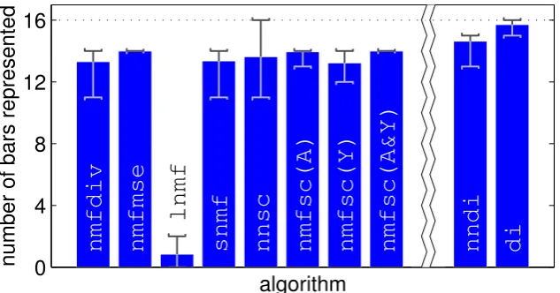
To provide a more realistic test, a new variation on the bars problem was used. In this version, training data consisted of 16 by 16 pixel images. Image components consisted of seven one-pixel wide bars and one nine-pixel wide bar in both the horizontal and vertical directions. Hence, as in previous experiments, there were eight image components at each orientation and 16 in total. Parallel bars did not overlap, however, the proportion of overlap between the nine-pixel wide bars and all other perpendicular bars was large, while the proportion of overlap between perpendicular one-pixel wide bars was less than in the standard bars problem. Each horizontal bar was selected to be present in an image with a probability of 18 while vertical bars occurred with a probability of 321. Hence, in this test case half the underlying image components occurred at a different frequency to the other half and two of the components were a different size to the other 14.
1k
1k 2k 3k
X
Y
X
X
Y
2kY
3kX4k
bar 1
bar 2
bar 3
Figure 9: An illustration of a the role of negative weights in the dendritic inhibition algorithm. Nodes are
shown as large circles, excitatory synapses as small open circles and inhibitory synapses as small filled circles. NodesY1kandY3kare selective for the double-width bars1and3respectively. The occurrence
in an image of the double-width bar ‘bar2’ would be indicated by both nodesY1kandY3kbeing active
at half-strength. However, if bar2occurs sufficiently frequently, the negative afferent weights indicated will develop which will suppress this response and enable the uncommitted node (Y2k) to compete to
respond to this pattern. Note that each bar would activate two columns each containing eight input nodes, but only one input node per column is shown for clarity.
0
4
8
12
16
number of bars represented
nmfdiv
nmfmse
lnmf
snmf
nnsc
nmfsc(A)
nmfsc(Y)
nmfsc(A&Y)
nndi
di
algorithm
Figure 10: Performance of each algorithm when trained on the unequal bars problem, with 32 basis
vectors or nodes, andp = 400. Each bar shows the mean number of components correctly identified by each algorithm when tested over 25 trials. Error bars show best and worst performance across the 25 trials.
(a) nndi
(b) di
Figure 11: (a) and (b) Typical recognition weights learnt by 32 nodes when both versions of the dendritic
inhibition algorithm were trained on the CBCL face database. Light pixels indicate strong weights.
3.5
Face Images
Previously, NMF algorithms have been tested using a training set that consists of images of faces (Lee and Seung,
1999;Hoyer,2004;Li et al.,2001;Feng et al.,2002). When these training images are taken from the CBCL face database1, algorithmnmfdivlearns basis vectors that correspond to localised image parts (Lee and Seung,1999;
Hoyer,2004;Feng et al.,2002). However, when applied to the ORL face database2, algorithmnmfmselearns global, rather than local, image features (Li et al.,2001;Hoyer,2004;Feng et al.,2002). In contrast, algorithm
lnmflearns localised representations of the ORL face database (Feng et al.,2002;Li et al.,2001). Algorithm
nmfsccan find either local or global representations of either set of face images with appropriate values for the
constraints on the sparseness of the basis vectors and activations. Specifically, nmfsclearns localised image parts when constrained to produce highly sparse basis images, but learns global image features when constrained to produce basis images with low sparseness or if constrained to produce highly sparse activations (Hoyer,2004). Hence, NMF algorithms can, in certain circumstances, learn localised image components, some of which appear to roughly correspond to parts of the face, but others of which are arbitrary, but localised, blobs. Essentially the NMF algorithms select a subset of the pixels which are simultaneously active across multiple images to be represented by a single basis vector. The same behaviour is observed in the bars problems, reported above, where a basis vector often corresponds to a random subset of pixels along a row or column of the image rather than representing an entire bar. Such arbitrary image components are not meaningful representations of the image data. In contrast when the dendritic inhibition neural network is trained on face images, it learns global represen-tations. Figure11a and Figure11b show the results of trainingnndianddi, for 10000 iterations, on the 2429 images in the CBCL face database. Parameters were identical to those used for the bars problems, except the weights were initialised to random values chosen from a Gaussian distribution with a larger standard deviation (0.005n
m) as this was found necessary to cause bifurcation of activity values. In both cases, each node has learnt
to represent an average (or prototype) of a different subset of face images. When presented with highly over-lapping training images the neural network algorithm will learn a prototype consisting of the common features between the different images (Spratling and Johnson,2006). When presented with objects that have less overlap, the network will learn to represent the individual exemplars (Spratling and Johnson,2006). These two forms of representation are believed to support perceptual categorisation and object recognition (Palmeri and Gauthier,
2004).
4
Discussion
The NMF algorithmlnmfimposes the constraint that the basis vectors be orthogonal. This means that image components may not overlap and, hence, results in this algorithm’s failure across all versions of the bars task. In all these tasks the underlying image components are overlapping bars patterns (even if they do not overlap in any single training image, as is the case with the one-orientation bars problem).
NMF algorithms which find non-negative factors without other constraints (i.e.,nmfdivandnmfmse) gen-erally succeed in identifying the underlying components of images when trained using images in which there is no occlusion (i.e., on the linear and one-orientation bars problems). However, these algorithms fail when
occlu-1CBCL Face Database #1, MIT Center For Biological and Computation Learning,
http://www.ai.mit.edu/projects/cbcl
2The ORL Database of Faces, AT&T Laboratories Cambridge,
sion does occur between image components, and performance gets worse as the degree of occlusion increases. Hence, these algorithms fail to learn many image features in the standard bars problem and produce even worse performance when tested on the double-width bars problem.
NMF algorithms that find non-negative factors with an additional constraint on the sparseness of the activations (i.e.,snmf,nnsc, andnmfsc (Y)) require that the rows ofYhave a particular sparseness. Such a constraint causes these algorithms to learn components that are present in a certain fraction of the training images (i.e., each factor is required to appear with a similar frequency). Such a constraint can overcome the problems caused by occlusion and enable NMF to identify components in training images where occlusion occurs. For example,
nnscproduced good results on the double-width bars problem. Given sufficient training data,nnscalso reliably finds nearly all the image components in all experiments except for the standard bars test whenn= 16and the unequal bars problem. However,nmfsc (Y)fails to produce consistently good results across experiments. This algorithm only reliably found all the image components for the standard bars problem whenn= 16and for the linear bars problem. Despite constraining the sparseness of the activations, algorithmsnmfproduced poor results in all experiments except for the linear bars problem.
The NMF algorithm that finds non-negative factors with an additional constraint on the sparseness of the basis vectors (i.e.,nmfsc (A)) requires that the columns ofAhave a particular sparseness. Such a constraint causes this algorithm to learn components that have a certain fraction of pixels with values greater than zero (i.e., all factors are required to be a similar size). This algorithm produces good results across all the experiments except the unequal bars problem. Constraining the sparseness of the basis vectors thus appears to overcome the problems caused by occlusion and enable NMF to identify components in training images where occlusion occurs. However, this constraint may itself prevent the algorithm from identifying image components which are a different size from that specified by the sparseness parameter. The NMF algorithm that imposes constraints on both the sparseness of the activations and the sparseness of the basis vectors (i.e.,nmfsc (A&Y)) produces results similar to those produced bynmfsc (A).
The performance of thenmfscalgorithm depends critically on the particular sparseness parameters that are chosen. As can be seen from figure12, performance on a specific task can vary from finding every component in every trial, to failure to find even a single component across all trials. While appropriate values of sparseness constraint can enable the NMF algorithm to overcome inherent problems associated with the non-linear superpo-sition of image components, inappropriate values of sparseness constraint will prevent the identification of factors that occur at a different frequency, or that are a different size, to that specified by the sparseness parameter cho-sen. This is particularly a problem when the frequency and size of different image components varies within a single task. Hence, thenmfscalgorithm was unable to identify all the components in the unequal bars problem with any combination of sparseness parameters (figure12d). In fact, no NMF algorithm succeeded in this task: either because the linear NMF model could not deal with occlusion or because the algorithm imposed sparseness constraints that could not be satisfied for all image components.
The parameter search shown in figure12was performed in order to select the parameter values that would produce the best overall results across all the tasks used in this paper for algorithmsnmfsc (A),nmfsc (Y),
andnmfsc (A&Y). However, in many real-world tasks the user may not know what the image components should
look like, and hence, it would be impossible to search for the appropriate parameter values. Thenmfscalgorithm is thus best suited to tasks in which all components are either a similar size or occur at a similar frequency, and for which this size/frequency is either known a priori or the user knows what the components should look like and is prepared to search for parameters that enable these components to be ‘discovered’ by the algorithm.
Sparseness constraints are also often employed in neural network algorithms. However, in such recognition models, sparseness constraints usually limit the number of nodes that are simultaneously active in response to an input image (F¨oldi´ak and Young,1995;Olshausen and Field,2004). This is equivalent to constraining the sparse-ness in the columns ofY(rather than the rows ofY, or the columns ofA, as has been constrained in the NMF algorithms). Any constraints that impose restrictions on the number of active nodes will prevent a neural net-work from accurately and completely representing stimuli (Spratling and Johnson,2004). Hence, such sparseness constraints should be avoided. The dendritic inhibition model succeeds in learning representations of elementary image features without such constraints. However, to accurately represent image features that overlap, it is neces-sary for negative weight values to be allowed. This algorithm (di) produced the best overall performance across all the experiments performed here. This is achieved because this algorithm does not falsely assume that image composition is a linear process, nor does it impose constraints on the expected size or frequency of occurrence of image components. The dendritic inhibition algorithm thus provides an efficient, on-line, algorithm for finding image components.
train-(a) (b) (c) (d)
Figure 12: Performance of thenmfscalgorithm across the range of possible combinations of sparseness parameters. For (a) the standard bars problem, (b) the one-orientation bars problem, (c) the double-width bars problem, and (d) the unequal bars problem. In each case,n= 32andp= 400. The sparseness ofY varies along the y-axis and the sparseness ofAvaries along the x-axis of each plot. Since the sparseness constraints are optional, ’None’ indicates where no constraint was imposed. The length of the edge of each filled box is proportional to the mean number of bars learnt over 25 trials for that combination of parameters. Perfect performance would be indicated by a box completely filling the corresponding element of the array. ‘X’ marks combinations of parameter values for which the algorithm encountered a division-by-zero error and crashed.
ing images contain virtually identical patterns of pixel values. These re-occurring, holistic patterns, are learnt by the dendritic inhibition algorithm. In contrast, the NMF algorithms (in certain circumstances) form distinct basis vectors to represent pieces of these recurring patterns. The separate representation of sub-patterns is due to con-straints imposed by the algorithms and is not based on evidence contained in the training images. Hence, while these constraints make it appear that NMF algorithms have learnt face parts, these algorithms are representing arbitrary parts of larger image features. This is demonstrated by the results generated when the NMF algorithms are applied to the bars problems. In these cases, each basis vector often corresponds to a random subset of pixels along a row or column of the image rather than representing an entire bar. Such arbitrary image components are not meaningful representations of the image data. Rather than relying on a subjective assessment of the quality of the components that are learnt, the bars problems that are the main focus of this paper, provide a quantitative test of the accuracy and reliability with which elementary image features are discovered. Since the underlying image components are known, it is possible to compare the components learnt with the known features from which the training images were created. These results demonstrate that when the training images are actually composed of elementary features, NMF algorithms can fail to learn the underlying image components, whereas, the dendritic inhibition algorithm reliably and accurately does so.
Intuitively, the dendritic inhibition algorithm works because the learning rule causes nodes to learn re-occurring patterns of pre-synaptic activity. As an afferent weight to a node increases, so does the strength with which that node can inhibit the corresponding input activity received by all other nodes. This provides strong competition for specific patterns of inputs and forces different nodes to learn distinct image components. However, because the inhibition is specific to a particular set of inputs, nodes do not interfere with the learning of distinct image components by other nodes. Unfortunately, the operation of this algorithm has not so far been formulated in terms of the optimisation of an objective function. It is hoped that the empirical performance of this algorithm will prompt the development of such a mathematical analysis.
5
Conclusions
to employ such constraints requires a priori knowledge, or trial-and-error, to find appropriate parameter values and can result in failure to identify components that violate the imposed constraint. In contrast, a neural network algorithm, employing a non-linear activation function, can reliably and accurately learn image components. This neural network algorithm is thus more likely to provide a robust method of learning image components suitable for object recognition.
Acknowledgements
This work was funded by the EPSRC through grant number GR/S81339/01. I would like to thank Patrik Hoyer for making available the MATLAB code that implements the NMF algorithms and which has been used to generate the results presented here.
References
Ahalt, S. C., Krishnamurthy, A. K., Chen, P., and Melton, D. E. (1990). Competitive learning algorithms for vector quantization. Neural Networks, 3:277–90.
Barlow, H. B. (1990). Conditions for versatile learning, Helmholtz’s unconscious inference, and the task of perception. Vision Research, 30:1561–71.
Barlow, H. B. (1995). The neuron doctrine in perception. In Gazzaniga, M. S., editor, The Cognitive Neuro-sciences, chapter 26. MIT Press, Cambridge, MA.
Charles, D. and Fyfe, C. (1997). Discovering independent sources with an adapted PCA neural network. In Pearson, D. W., editor, Proceedings of the 2nd International ICSC Symposium on Soft Computing (SOCO97). NAISO Academic Press.
Charles, D. and Fyfe, C. (1998). Modelling multiple cause structure using rectification constraints. Network: Computation in Neural Systems, 9(2):167–82.
Davies, G. M., Shepherd, J. W., and Ellis, H. D. (1979). Similarity effects in face recognition. American Journal of Psychology, 92:507–23.
Dayan, P. and Zemel, R. S. (1995). Competition and multiple cause models. Neural Computation, 7:565–79. Feng, T., Li, S. Z., Shum, H.-Y., and Zhang, H. (2002). Local non-negative matrix factorization as a visual
representation. In Proceedings of the 2nd International Conference on Development and Learning (ICDL02), pages 178–86.
F¨oldi´ak, P. (1989). Adaptive network for optimal linear feature extraction. In Proceedings of the IEEE/INNS International Joint Conference on Neural Networks, volume 1, pages 401–5, New York, NY. IEEE Press. F¨oldi´ak, P. (1990). Forming sparse representations by local anti-Hebbian learning. Biological Cybernetics,
64:165–70.
F¨oldi´ak, P. and Young, M. P. (1995). Sparse coding in the primate cortex. In Arbib, M. A., editor, The Handbook of Brain Theory and Neural Networks, pages 895–8. MIT Press, Cambridge, MA.
Frey, B. J., Dayan, P., and Hinton, G. E. (1997). A simple algorithm that discovers efficient perceptual codes. In Jenkin, M. and Harris, L. R., editors, Computational and Psychophysical Mechanisms of Visual Coding. Cambridge University Press, Cambridge, UK.
Fyfe, C. (1997a). Independence seeking negative feedback networks. In Pearson, D. W., editor, Proceedings of the 2nd International ICSC Symposium on Soft Computing (SOCO97). NAISO Academic Press.
Fyfe, C. (1997b). A neural net for PCA and beyond. Neural Processing Letters, 6(1-2):33–41.
Ge, X. and Iwata, S. (2002). Learning the parts of objects by auto-association. Neural Networks, 15(2):285–95. Harpur, G. and Prager, R. (1996). Development of low entropy coding in a recurrent network. Network:
Compu-tation in Neural Systems, 7(2):277–84.
Hinton, G. E., Dayan, P., Frey, B. J., and Neal, R. M. (1995). The wake-sleep algorithm for unsupervised neural networks. Science, 268(5214):1158–61.
Hinton, G. E. and Ghahramani, Z. (1997). Generative models for discovering sparse distributed representations. Philosophical Transactions of the Royal Society of London. Series B, 352(1358):1177–90.
Hochreiter, S. and Schmidhuber, J. (1999). Feature extraction through LOCOCODE. Neural Computation, 11:679–714.
Hoyer, P. O. (2002). Non-negative sparse coding. In Neural Networks for Signal Processing XII: Proceedings of the IEEE Workshop on Neural Networks for Signal Processing, pages 557–65.
Jutten, C. and Herault, J. (1991). Blind separation of sources, part I: an adaptive algorithm based on neuromimetic architecture. Signal Processing, 24:1–10.
Kohonen, T. (1997). Self-Organizing Maps. Springer-Verlag, Berlin.
Lee, D. D. and Seung, H. S. (1999). Learning the parts of objects by non-negative matrix factorization. Nature, 401:788–91.
Lee, D. D. and Seung, H. S. (2001). Algorithms for non-negative matrix factorization. In Leen, T. K., Dietterich, T. G., and Tresp, V., editors, Advances in Neural Information Processing Systems 13, Cambridge, MA. MIT Press.
Li, S. Z., Hou, X., Zhang, H., and Cheng, Q. (2001). Learning spatially localized, parts-based representations. In Proceedings of the IEEE Conference on Computer Vision and Pattern Recognition (CVPR01), volume 1, pages 207–12.
Liu, W. and Zheng, N. (2004). Non-negative matrix factorization based methods for object recognition. Pattern Recognition Letters, 25(8):893–7.
Liu, W., Zheng, N., and Lu, X. (2003). Non-negative matrix factorization for visual coding. In Proceedings of the IEEE International Conference on Acoustics, Speech and Signal Processing (ICASSP03), volume 3, pages 293–6.
L¨ucke, J. and von der Malsburg, C. (2004). Rapid processing and unsupervised learning in a model of the cortical macrocolumn. Neural Computation, 16(3):501–33.
Meila, M. and Jordan, M. I. (2000). Learning with mixtures of trees. Journal of Machine Learning Research, 1:1–48.
Oja, E. (1992). Principal components, minor components, and linear neural networks. Neural Networks, 5:927–35. Olshausen, B. A. and Field, D. J. (2004). Sparse coding of sensory inputs. Current Opinion in Neurobiology,
14:481–7.
O’Reilly, R. C. (2001). Generalization in interactive networks: The benefits of inhibitory competition and Hebbian learning. Neural Computation, 13(6):1199–1242.
Palmeri, T. J. and Gauthier, I. (2004). Visual object understanding. Nature Reviews Neuroscience, 5(4):291–303. Plumbley, M. D. (2001). Adaptive lateral inhibition for non-negative ICA. In Proceedings of the international
Conference on Independent Component Analysis and Blind Signal Separation (ICA2001), pages 516–21. Saund, E. (1995). A multiple cause mixture model for unsupervised learning. Neural Computation, 7(1):51–71. Sinha, P. and Poggio, T. (1996). I think i know that face...,. Nature, 384(6608):404.
Spratling, M. W. and Johnson, M. H. (2002). Pre-integration lateral inhibition enhances unsupervised learning. Neural Computation, 14(9):2157–79.
Spratling, M. W. and Johnson, M. H. (2003). Exploring the functional significance of dendritic inhibition in cortical pyramidal cells. Neurocomputing, 52-54:389–95.
Spratling, M. W. and Johnson, M. H. (2004). Neural coding strategies and mechanisms of competition. Cognitive Systems Research, 5(2):93–117.