A Unified Newtonian Relativistic Quantum Resolution of the Supposedly Missing Dark Energy of the Cosmos and the Constancy of the Speed of Light

A Unified Newtonian-Relativistic Quantum Resolution

of the Supposedly Missing Dark Energy of the Cosmos

and the Constancy of the Speed of Light

M. S. El Naschie

Department of Physics, University of Alexandria, Alexandria, Egypt Email: [email protected]

Received November 16, 2012; revised December 22, 2012; accepted December 31, 2012

ABSTRACT

Time dilation, space contraction and relativistic mass are combined in a novel fashion using Newtonian dynamics. In this way we can surprisingly retrieve an effective quantum gravity energy-mass equation which gives the accurate ex- perimental value of vacuum density. Furthermore Einstein’s equation of special relativity E = mc2_{, where mis the mass}

and c is the velocity of light developed assuming smooth 4D space time is transferred to a rugged Calabi-Yau and K3 fuzzy Kähler manifolds and revised to become _E

 

_mc2

 

_{22 , where the division factor 22 maybe interpreted as the}

compactified bosonic dimensions of Veneziano-Nambu strings. The result is again an accurate effective quantum grav- ity energy-mass relation akin to the one found using Newtonian dynamics which correctly predicts that 95.4915028% of the energy in the cosmos is the hypothetical missing dark energy. The agreement with WMAP and supernova meas- urements is in that respect astounding. In addition different theories are used to check the calculations and all lead to the same quantitative result. Thus the theories of varying speed of light, scale relativity, E-infinity theory, M-theory, Het- erotic super strings, quantum field in curved space time, Veneziano’s dual resonance model, Nash Euclidean embedding and super gravity all reinforce, without any reservation, the above mentioned theoretical result which in turn is in total agreement with the most sophisticated cosmological measurements which was deservingly awarded the 2011 Nobel Prize in Physics. Finally and more importantly from certain viewpoints, we reason that the speed of light is constant because it is a definite probabilistic expectation value of a variable velocity in a hierarchical fractal clopen, i.e. closed and open micro space time.

Keywords: Dark Energy; Homology of Fuzzy Kähler; Betti Numbers; Heterotic Strings; Revised Special Relativity;

Speed of Light as a Probabilistic Expectation Value

1. Introduction

The present work is mainly concerned with devising a theoretical explanation for the mystery of the so-called missing dark energy of the cosmos [1-4]. However this is all linked to quantum gravity [1-23] and we start here from special relativity and address the greatest puzzle of them all which we invariably took and rather wrongly as a given experiential fact of Nature which cannot be re- duced or interrogated any further namely the constancy of the speed of light. As is well known Einstein’s special relativity presupposes a smooth space time with Lor- entzian symmetry group invariance [1]. Quantum space time on the other hand is modeled via radically different geometrical visualization [1-8]. In string theory, M-the- ory and super gravity one uses various types of Calabi- Yau and complex Kähler manifolds for space time extra dimensions [9-17]. Consequently requiring the Poincaré

invariance in a complex space with such extra and com- pactified dimensions will most definitely lead to a dif- ferent energy-mass relation than the classical famous Einstein equation of special relativity. On the other hand should the principle of scale relativity hold, then one would expect to retrieve Einstein’s familiar formula in a scaled form [3-5]. In a sense we expect a type of scale similarity close to that found between Newton’s kinetic energy and the famous energy-mass formula of relativity which differs by a factor of only 1/2 and changing the variable velocity v to the puzzlingly constant speed of light c. Noting that for a continuous manifold the Betti number 2which counts the three dimensional holes in a

manifold is given by ₂ b

1

b  and that the same Betti number for a K3 Kähler is ₂ , it is possible to show that E = mc2 _{may be elevated to quantum relativ-}

ity, i.e. an effective quantum gravity equation when scaled by

22 b 

   

2 3 2 3 1

QRb S b K  22

This prior intuitive mathematical expectation was con- firmed on two counts, namely first experimentally using the WMAP and supernova cosmic measurements [4,19] and second theoretically using numerous sophisticated established theories, all leading to the same robust result, namely a scaling factor 1 22 (see Table 1) [24-26].

In this paper we start first from basic principles con- nected to special relativity then transform these princi- ples back to Newtonian dynamics only to obtain quantum relativity results. Surprisingly that way we retrieve a highly non-classical equation indeed combining the quan- tum with relativity via a four dimensional Hilbert-He hy- percube [7] (see Overview 3 and Table 2).

Subsequently we show that for a fuzzy Kähler [10,13] the scaling factor changes from 1 22 to 1 22



k









1 22.18033989 . In addition to giving a derivation of the new quantum relativity equation

 

2

QR

E  mc where m is the mass and c is the speed of light, we show that this result is in exquisite agreement with the cosmo- logical measurement of COBE and WMAP as well as the analysis of certain supernovas which led to the award of last year’s 2011 Nobel Prize in Physics [4,18]. Based on our K3 fuzzy Kähler we can predict with very high preci- sion that the percentage of hypothetical dark energy, supposedly missing, in the universe is 95.4915028%. This is a probably unprecedented agreement between the- ory and measurement in cosmology [4], if not in all of theoretical physics [1]. We will hopefully know with absolute certainty when the Planck measurement project [18] is completed.

Last but as we mentioned above by no means least, noting that all real measurements are taken in the expec- tation dimensionality of spacetime DT 4 and DH 

, we reason that the speed of light is constant because it is the probabilistic expectation value of variable speed in a fractal spacetime. In other words the constancy of the experimental value of the speed of light is the evidence that our spacetime manifold is highly complex non-classical fractal-Cantorian manifold on the quantum scale. Consequently this space must be topo- logically clopen i.e. closed and opened at the same time.

3

4 4.23606

2. Motives for Revising Einstein’s

Energy-Mass Equation—Combining

Newtonian, Relativistic and Quantum

Mechanics

2.1. General Remarks and Topological Considerations

An equation based entirely on the tacit assumption of a smooth space with Lorentzian space time invariance de- veloped many years before the standard model of high energy particle physics and quantum field theory were discovered [1] could not possibly be expected not to

break down at some quantum or intergalactic scales [1-3, 19]. The above is an accurate description of the circum- stances surrounding the inception of A Einstein Iconic formula E = mc2 _{of special relativity in 1905. In the pre-}

sent paper we show that the supposedly missing dark energy in the cosmos, discovered through various accu- rate cosmological measurements [4] is in effect due to some basic fundamental inadequacies of applying Ein- stein’s celebrated equation E = mc2 _{(where E is the en-}

ergy, mis the mass and c is the speed of light) outside its range of validity [5,6]. We thought for a long time and understandably so that gravity cannot have that crucial effect on elementary particle physics [1]. Similarly we thought that quantum mechanics also has very little ef- fect on cosmology except maybe when it comes to in- credibly shrinking objects such as black holes [1]. How- ever when we started asking very deep questions regard- ing the unification of all fundamental interactions [7,8] we recognized suddenly that at the extreme small dis- tances such as the Planck length (10−33 _{cm) the feeble}

gravity becomes as strong as the other three fundamental forces, i.e. the weak force, the strong force and the elec- tromagnetic force [1,3,7]. On the other hand we have now just realized that quantum effects, such as quantum entanglement, have an equally huge impact on physics at extremely large intergalactic distances. It is so profound that the classical equation of Einstein E = mc2 _{is off the}

correct result by almost 95.5% [4,19]. Seen with the eyes of a particle physicist this should not be that astonishing because the only degree of freedom of special relativity is a single messenger particle, the photon [1]. By contrast the simplest model for high energy quantum physics, the standard model, requires 12 photon-like messenger parti- cles equivalent to 12 degrees of freedom i.e. 12 general- ized coordinates in the corresponding Lagrangian [1,7]. Special relativity therefore is highly confined by the Ray- leigh theorem on Eigen values and is bound to over-es- timate the energy levels.

In the present work we trace back the shortcoming in and prove that this is the case because of the real non-classical geometry and topology of the actual fabric of space time [2,7,8]. This non-classical topology is essentially the cause of amplifying what we perceive as quantum effect which screens the energy by as much as 95.5% in full agreement with measurements [4]. In particular we will show that the ratio of the two Betti numbers [9-12] fixes the homology of space time’s de Rham topology of smooth classical space time of relativ- ity and the rugged K3 Kähler [11] based quantum space time of quantum gravity and give us a Weyl-Nottale scal- ing λ = b2 (smooth)/b2 (Kähler) equal to 1/22 which ac- counts for the 95.5% missing dark energy [4]. It is well known that the Betti numbers are topological invariants of a manifold [9,10] exactly he dimensions and the

2

E mc

Table 1. The Energy mass relation of quantum relativity using various fundamental theory.

Theory Mass-energy equation Remarks

Newton 1 2

2 N

E  mv V is velocity, m is mass

Special relativity 2

R

E mc C is the speed of light, i.e. photons 0

1) Quantum relativity: fusing quantum entanglement P(Hardy) and special relativity as well as Newtonian mechanics

   

 





2

2 2 5 5 2

1 Hardy 2 1 1 Hardy 2 2 2 NQR

E m v c P

mc P mc  mc

 

_  _

 

  

_Hardy 5

P  where 2



5 1



is the

golden section 0.6180338 For m c 1

we find PHardy2E where Eis Einstein’s maximal energy.

2) Combining general relativity and Yang-Mills three photons. This is basically a quantum field theory in curved space





 



 



2 4 2 2 1 1 1 1 20 1 1 22

o QR mc E R mc mc             

Yang-Mills predicts three photons, two are electrically charged and the third one is our familiar neutral photon. Here we are working with an effective quantum gravity action.

3) Special relativity in K3 Kähler

        2 2 2 2 2 special relativity 3 Kahler 1 1 22 22 b m E b K mc mc   

c K3 Kähler is a complex manifold with 4

complex dimensions used for compactification in superstring theories. The Betti Number b2 is

index counting 3-D holes. Betti numbers as

well as dimensions and the Euler characteristic fix homology of manifolds.

4) Relativity plus standard model plus Newtonian mechanics

 

     2

2 2

1 1

2

3 2

1 1 1

11 2 22

U E m SU SU mc mc    _{ }        _{  } _{ }     

v c

The standard model has no gravity and 12 massless gauge bosons. Adding the graviton we have 13 and subtracting the photon we are left again with our initial 12. Dividing U 1 by

 3 ,   2 , 1

SU SU U  means we are left with

11 isometrics i.e. particles.

5) General relativity plus holographic boundary      



   



    4 4 2 4 4 2 2 2,7

20 4 1

336 20 4 22

R D E

SL R D mc mc  _            mc    

 4

R is the number Independent Components of the Riemanian Tensor in D4 or the degrees of freedom of pure Gravity in D8

thus we have





      2 2 2 4 1 12

16 1 12 20.

n

R n n



 

 

6) General relativity plus 6D Calabi-Yau manifold

   





 

 

2

4 6 4

2 2

1

1 1

20 6 4 22

E m

R D D mc mc



 

 

 

c Calabi-Yau manifold has 6 real dimensions

and is used as K3 Kähler in superstring theories. By contrast K3 Kähler has 4 Dimensions only but they are complex dimensions, not real.

7) Special relativity in a hyper 4D J. Huan he Hilbert cube given by

3

1

4 4 4.2360679

1 4

4

D     

 2

_

_

2 5

1 1

2 2 1

E  mc 

 

 



1 1 

2

mc we introduced a light cone speed  

as well as a light cone mass



1  m  .

8) Nottale’s scale relativity

2 1 GUT E m n     

  c where GUT110 is the

inverse coupling constant of grand unification of all non-gravitational forces. Thus

  2 2 2 2 1 22.09 22 4.70042 mc mc

E  mc

Continued

9) Relativity plus 11 D-M theory plus super symmetry. This is effectively a

super-symmetric Penrose quasi crystal universe    

2 2

1 1

11 11 11 11 22

E mc D D       1 mc 

The isomorphic length of an 11 dimensional Penrose fractal universe is 22k 2 11



3



3



22 K 4  5

where     This is a

super symmetric Penrose tiling. Note that

3

4_{ is bosonic and 5}3_{is fermionic}

tiling dimension

10) Relativity plus fractal Witten M-theory

plus Newtonian mechanics  

 

2 5 2

5

1 1 1

11 2 2

E m v c 



   

_{ }  _{ }

  

  mc

Fractal M-theory is dimension

11 11 11  k 2 _{where k}3



_13



and thus _{k 2}5_.

11) Fractal standard model plus relativity plus

Newtonian mechanics









2 2 2 5 2 1 22 2 2 22.18033989 o o mc E k mc mc        _{  }       

mc The fractal weight of the 12 particles of the

standard model is  o 11.70880393 and represents 14 particles. The fractal weight of a photon is   0.61803398.

12) Relativity plus E8E8 exceptional Lie

symmetry groups _{     }

2

2

2 2

1 8 8

496 3 2 1

1 1

22 496 12

E mc

E E SM mc SU SU U

mc mc           

When Einstein drove his famous formula

2

E mc high energy Physics was at it’s very beginning and only two elementary particles were known, the photon and the electron. To extend the range of validity of Einstein’s formula a minimum of 12 massless gauge bosons are needed. This could be however extended to 496 massless gauge bosons in case of E8E8 or SO(32) superstring theory.

13) Varying speed of Light Theory of Magueijo and Smolin

2 2 1 P mc E mc E  

Transferring to unit the interval

one finds _Hardy 5

P

E P 

Sigalotti Cv 

Kaluza-Klein dimension KK 5

mm D 

    

 

 





2 2

5

2 5

5 1 21

1

22 2

mc mc

E

K

mc K mc

       

   2

The same result may be obtained by noting

that 2

P

mc E

 could be expressed in any of

the following terms

  No 8064 21, 2,7 48 SL    

 _2,7  6 _{336 105 21}

SL R      ,   8 5 5 i E SU





, 504 24 21 Note

that 5

P

E  means that Hardy’s quantum

entanglement of two particles constitutes the maximum unit of Planck energy which is intuitively understandable in view of Witten T-duality

14) Conjectured E12 exceptional Lie group

and Calabi-Yau Manifold with Euler

characteristic equal 200  4

CP   

2 2

2 2

57 12 200

12 22 684 200 mc mc E E mc mc         12 684

E  is close to, 17

1

stein686



,

where stein stands for the dimensions of two and three stein spaces. There are only 17 of them.

15) Lagrangian multiplier method for isoparametric variational problems

2 1 2

2

Va _ mv G_

  Where  is the

Lagrangian multiplier and

consequently

steady state is given by

11 0 0

12 1 11 i

G



    

2

 v0 which leads

for vcto 1 2  _{11 0}

2mc   or

2

22

mc

 .

Thus  can be interpreted as EQR

The quadratic form of V is given

Continued

16) Theory of probabilistic special relativity

1 1 n

P  

  

 is general Cantorian-fractal

probability which for n2 and  

gives _P_Hardy_5 _{of quantum}

entanglement. Thus we have 21

1

m  m

  

 ,

21

1

x  x

  

 ,

21

1

t  t

  

 from

 2

1 2

E m v c and minimizing one finds



5 ₂

 

2 E mc

The minimization of P leads to

   

1 1 d

0

2 d 1

n 



 

 _

 . For n2 one finds

2 _{1 0}

    i.e.   ₁ , ₂ 1 where



5 1 2



  The general expression is

2 2

1 1

.

2 1

E  m

  

 c For   we find the

exact E namely





2

22

mc c 5 ₂ 2

E m

K



 

 where _K3



_13



_{0.18033989}

17) General relativity-super gravity

We start by _2Rn4_{of the Riemenian Tensor.}

This is . By contrast the

number of independent components taken into account by A. Einstein is

 4 _4 ₅₁₂

s

R 

 

 2 4 

 4 _{ 4}2



₄2_{1 12 20}



_

R Thus

1 1

22.18107301 512 20

 

 and

 



2

2 5 ₂

22.1810703

mc

E mc 

The analysis is quite similar to when we use

E8E8. We recall that in this case we have

 





4

5

1 1

496 4 8 8

1 1

2 22.1810703 492

E E D





 

 

 

which is the same result obtained using general “super symmetric” relativity or super gravity.

Space time dimensions and energy in the three fundamental theories: classical, relativistic and quantum gravity.

Euler characteristics [9-12] with the added advantage that

b2 counts what we may call three dimensional holes (voids) [9] in the manifold which in this case is our real space time fabric. That way all the fractal-like fine struc- tures of our space are taken into account [9,13]. How this actually is done is what we will explain next.

Dimensions of real space (D)

Energy-mass-equation (E)

2 Emc



5 1 2



 

E = Energy

M = Mass

γ = Lorentz factor

However before going ahead with the preceding out- lined topological geometrical program, we will regress to reconsider relativity and Newtonian dynamics at the most possible basic level [1,20,21]. In the course of doing that, we will arrive at a far reaching conclusion with tremen- dous impact on the entire foundation of physics namely that the constancy of the speed of light and similar to

and of space time (see

Overview 1) is a consequence of the fractal Cantorian

nature of the very fabric of space and time. Consequently the speed of Light is simply an expectation value in the sense of probability theory of an otherwise varying speed.

4

T

D  D_H 4.236067977

2.2. Basic Principles of Special Relativity Starting from Newtonian Dynamics and Leading to Quantum Mechanics and Quantum Relativity [20] (see Overview 2)

We will not start here from of relativity but rather from Newtonian kinetic energy

2

E mc

 

_{1 2} 2

E mv . Overview 1.

Now we ponder the three well known relativistic effects, namely 1) time dilation which we introduce here by a simple factor 1 leading to tt



1



2) Then we have space contraction which is obviously X



1



where X is a space coordinate. Finally we have increased mass as vcand this leads to 3) relativistic mass



1



m  . Consequently our _E

 

_{1 2 mv}2 _becomes

 

_{1 2 1}



1 2 2

1

E   m

   

  _{ }



  c



(1) The factor



1

 

2 1 will play a crucial role in our theory leading to the inescapable conclusion that space time of special relativity is a random Cantorian Fractal with an average expectation value for the speed of Light.

Let us see what value this twisted boost 1 and anti-boost 1 must take in order to retrieve Newton’s energy and Einstein’s energy. In the case of Newtonian energy, this is very simple because we must have









2 1

1 1

  



 (2) from which one finds that either   10 or  

2 3

  to obtain _E

 

_{1 2 mv}2_{. Note that  3 should} be interpreted as the natural classical space which is not 4D but 3 + 1 dimensional space where time is now a simple parameter. For the relativistic case on the other hand, things are far more interesting and revealing be- cause we must have









2 1

2 1

  



 (3) This leads to a quadratic equation

2 _{4 1}

   0 (4) with two solutions [7,17]

3

1 4 4.236067977

    (5) and [7]

3

2 0.236067977

     (6) where 



5 1 2



. Both 1 and 2 lead to E = mc2_{. On the other hand 4}3 _{is the Hausdorff dimen-}

sion of a Hilbert-fractal hyper cube discussed extensively by Ji-Huan He and the author [7]. This is indeed more than a remarkable result linking for the first time fractals in the form of a Hilbert-He 4 dimensional hypercube and

The new Heuristic Lorentz transformation of E-infinity theory. We have boost 1 and anti-boost 1.

Relativity strange effects:

1) The mass increase as VC.

2) Time slows down as VC.

3) Rods become shorter as VC.

These effects lead to:

1 

mm  equivalent to light cone mass

   

1 1

t t X X

 

  _



  _ equivalent to light cone velocity

The Newtonian kinetic energy EN then becomes

      

2

2 2

2

2

2 2

1

1 1₁

2 2 1

1 1 2 1

N QR

QR QR

E mv E m

E mc mc

 



 _





   

 

 



c

This QR turned out to be 1 22 , for the Sigalotti Critical

value   where 2



5 1



Overview 2.

E-Infinity World Formula

In general:     

2

2

1 1

m 2 1 QR

E  v

 

 

 c where 1 is boost and 1 is anti boost

1) Newton 1 2

2

E mv 2) Einstein _{E mc} 2 _{3) E-infinity theory E}



_5 ₂



_mc2

We obtain a quadratic equation with two

solutions: 10 or i.e.

3



2 3

 

space

D

We obtain quadratic equation with two

solutions: 3

1

1 4 1

4 ₁

4 4

   

 



Note that 4-D J-Huan He-Hilbert hypercube

is of dimension 11 4 3. The second

solution is 3

2

   where 2



5 1



and  2 3

c

d _ _{i.e. negative topological}

dimension n 2

Also a quadratic equation with two solutions:

1 0

  or ₂ 1 1 1.472135856

1 2

10

k

   _ 



where _K3



_13



_{0.18033989}

For “natural” units m = c = 1 we have 1

2 QR

E  P(Hardy of quantum entanglement) and PImmirzi of loop quantum gravity   



P Hardy .



Thus E-infinity world formula says for   and m = c = 1 we find _Hardy1   5 ₂

2

E P 

special relativity [7]. This implies indirectly that the speed of light varies between Zero and Infinity with the familiar experimental value being simply the probabilis- tic expectation value. In the rest of this paper we will show how the factor



1

 

2 1



will lead to a quantum gravity-like equation combing relativity with quantum entanglement for the Sigalotti critical value



5 1 2



   [17,22,27,28]. The preceding results are once more neatly summarized in Overview No. 3.

3. Homology of a Space Time Based on

Crisp K3 Kähler Manifold [10]

Following super strings and related theories [12] we look first at the possibility of a quantum gravity spacetime based upon a K3 Kähler manifold [13]. We start with a non-fuzzy crisp Kähler then look at the fractal-like fuzzy case.

3.1. Classical Non-Fuzzy Kähler

We consider a K3 Kähler manifold with four complex dimensions used extensively in theories with hidden di- mensions particularly super and Heterotic string theory [12,13]. The manifold is fixed by the Betti numbers which determine the Euler characteristic and the signa- ture. In the case of non-fuzzy (crisp) K3 the Betti num- bers are [10,13]

0 4 1, 1 3 0, 2 19

b b  b b  b  and b2 3. (7) _

It follows then that the Euler characteristic is [10,13]

0 4 2 2 1 1 19 3 24

b b b b

_{  } _  _{     (8)} while [10,13]

2 2 2 3 19 22

b _b_b _{   (9)} and the signature is [10,13]

2 2 3 19 16

b b

 _ _ _{    . (10)} We stress once more that b2 counts the 3 dimensional holes in K3 and will play a crucial role in our derivation. 3.2. Fuzzy, Fractal-Like K3 Kähler

Now we look at an even more exotic version of K3 [13]. With that we mean fuzzy Kähler which we used in earlier studies in a slightly modified form [13,14]. The Kähler we construct here is a fuzzy version of the one consid- ered above. The K3 Kähler in question is given by the same 0 4 1 and b3 as the previous crisp Kähler. Only 2 and b2 which measure a sort of average number of

3D fractal voids are given by [13,14,24-26]. , ,

b b b 

b

6 2 19

b   and 3 2 3

b   (11) where 



5 1 2



. It follows then that [13,14]



6



3

2 19 3 22 22.18033989

b       k . (12)

It is important to note the following. The small num- bers _6 _{= 0.05572809014 as well as }3 _{= 0.236067977}

and _K3



_13



_{0.18033989 all have various physi-} cal, topological and geometrical interpretations. For in- stance _6 _{is the exact value of the vital Immirzi parame-}

ter of loop quantum gravity without which nothing would fit in this theory [15]. In addition _6 _{may be viewed as}

the probability for quantum entanglement of three quan- tum particles while _5 _{is the well known Hardy’s ge-}

neric probability of quantum entanglement [16,17,22] for two particles which was also confirmed experimentally. Thus _6 _{could be named the probability of Immirzi}

quantum entanglement. The _3 _{on the other hand is the}

generic probability of a Cantorian spacetime with a core Hausdorff dimension equal to



_43



_{ 4 4 and is} directly connected to the Unruh temperature [13] (see

Overview 4).

Finally,

3

1

10 2

k 

 _

. (13) That means

3

5

K  1 (14)

4. Elevating Einstein’s Relativistic Equation

to a Quantum Gravity Energy-Mass

Relation

We said that b2 is an important homological invariant of a manifold [9-11] and that it basically counts the 3 di- mensional voids in the manifold [9,14]. For a two sphere

S2 _{or any connected manifold b2 is equal to unity b2 = 1.}

On the other hand for our classical Kähler b2 = 3 + 19 = 22, and this number already indicates that this manifold is almost a Swiss cheese full of 3 dimensional holes [10, 13]. Compared to the smooth S2 _{manifold akin to the}

space time of Einstein, K3 has 22 times less space time and following general relativity, less energy [1]. Now following for instance Nottale’s scale relativity principle [24-26] we could define a scaling  to account for fractal voids to be









2 2

Einstein space 1

Kahler 22

QR

b b

   (15)

and use it to scale _{E mc} 2 to

 

 

2 2

2

1 22 0.0454545 .

QR QR

E mc m

mc

  

 _{  }

  

c

(16)

This implies that the missing hypothetical dark energy s

Fundamental Results

(A World Formula for mc2 _{= 1)}

 

 

1









P E-infinity General expression for quantum entanglement in cantorian spacetime of E-infinity where 2 4 5 1

n 

 

   

  _   

 

1) P(E-infinity) = _n2 _{P(Hardy’s two particle quantum entanglement)}

2) P(E-infinity) = _n3 _{P(The immirzi parameter of loop quantum gravity interpreted as a 3 particle quantum entanglement)}

3) P(E-infinity) = _n O _{P(Unruh temperature)}

4) P(E-infinity) = _n _{Zero(Classical world means no entanglement at all)} Important Notes:

Einstein’s equation _{E mc} 2 could be interpreted as describing a compactified modular curve with _{v c being the holographic horizon.} Similarly but in a complimentary way a random cantor set has a horizon namely a maximal Hausdorff dimension d_Hmax where





2 1 5

   . This corresponds to in relativity. Fusing the two modular spaces, the isomorphic length is found to be the

thought-after energy-mass relationship for quantum relativity

max V C

 

 

_{ }

2 5 _{2 .}

_

2

R Q

QR

E P

E mc 

 

This result means that 95.4915028 percent of the energy in the universe is either dark energy and dark matter or is not there at all. This quantitive result is in an almost perfect agreement with accurate cosmic measurement and super nova analysis of cosmic WMAP data.

Overview 4.



dark



1 1

 

100 95.454545% 22

E  _ _ 

  . (17)

This is extremely close to the cosmological measure- ment [4]. Even better still, if we use the fuzzy version of

K3 we arrive at a mathematically exact expression



dark



1 1

 

100 95.49150281%.

22

E

k

 

 _{ } 



  (18)

In fact when using the fuzzy Kähler, we notice imme- diately a quantum mechanical interpretation of the result because



2

1 22

QR

E

k

 

 _{ } _ mc



(19) means that

  

5

1 2

QR

E   _mc2 _{. (20)}

However _5 _{is nothing else but Hardy’s generic}

quantum entanglement of two quantum particles [16,17] so that our QR may be viewed as the screening of a

substantial part of the energy in the cosmos by quantum entanglement reducing the Newtonian action at distance by as much as



_15 _{2 100}



 

_{95.4915%. Finally} there is an even more immediate interpretation when we invoke string theory and M-theory as shown in Figures 1

and 2. In the case of string theory, we could argue our

case as following: The largest number of dimensions in Heterotic string theory is 26 in the classical case and 26 +

k in the transfinite fractal-fuzzy case. However we can make measurement only via 4 dimensions, 3 space di- mensions and one time dimension. Thus we have 22 hid- den dimensions [12]

5

Hardy's

-Quantum Entanglement



5

11-Dimensional Hilbert Cube

1

11 ₁

11 11 11 

 



  

[image:8.595.310.536.305.494.2]

Witten's 11-D M-Theory

Figure 1. Combining M-theory and quantum entanglement to give a fractal M-theory.

Where 11 is Witten’s M-theory dimension and _115_15 _is

the spacetime dimension of Witten’s fractal-like M-theory

  

2 5



2

1 11

1 11

1 ₂

1 2

11 1 11

QR

E m 

  

 

_{ } 

 

 _  

  _{ } 

 

 

 _{ }  _ 

   

 

 _{ } 

 _{ } 

   

 

 



c mc

Here  



5 1 2



and compactified

“dark” dimensions, m is the mass and c is the velocity of light.

 26  4 _{26 4 22}

D D   

[image:8.595.310.537.535.695.2]



hidden



26 4 22

D    (21) or more accurately [12,14]



hidden



26 4 22

D    k k. (22) Thus our scaling exponent is





1 hidden 1 2

QR D

   2



(23) Or in the fuzzy case [13,14]



1 22

QR k

   . (24) Within this mental picture we could say that the miss- ing dark energy is concealed and hidden inside the dark extra dimension [7,12,14]. Now all what we need to do in order to see this unified picture of Newtonian, relativistic and quantum dynamics is to set following Sigalotti [27, 28]  



_{1 }



2



in our expression of Section 2.2 and find that _{1 }



_5

 _{ } _



_

_

 2and that is exactly equal 1 22k and in addition _5 _{is Hardy’s generic prob-}

ability of quantum entanglement [16,17,22].

Incidentally _5 _{could be also interpreted as a dimen-}

sionless Planck energy equal to EP of the theory of vary-

ing speed of Light [5,6] while _3 _{is corresponding to the}

Unruh temperature (See Overview 4) as mentioned ear-

lier [29]. There is a fundamental connection between what we may call Witten Hyper cube and Witten Fractal M-Theory connecting quantum relativity with Hardy’s Quantum Entanglement. This is represented in a diagram and outlined in Figures 1 and 2. In Table 1 we summa-

rized the result of applying 17 methods and theories to the problem at hand showing that the reduction factor in E is invariantly  1 22

o

.

5. Special Relativity Gauged via Yang-Mills

Theory Leads to Quantum Gravity

In what follows we show how to obtain the preceding result using a direct comparison between the field stren- gth of Yang-Mills theory and that of special relativity [1]. In doing that we have de facto produced an effective quantum gravity equation [20]. Now special relativity spacetime is flat. The four types of photons namely are assumed for the moment to be all massless and cannot curve space time [1]. By contrast the Yang-Mills field has a field strength [1] given by and can easily be shown to be at the point of grand uni- fication energy scale

, , ,

o _{W W}

  _

2

8π

  

2 g

F  where _g 42 is the inverse common group coupling of GUT [1,7]. Field strength in the terminology of fiber bundle theory is sim- ply the curvature [1]. Thus although the space of Ein- stein’s relativity is flat, it does have 4 photon-like gauge Bosons given by U

 

1 SU

 

2   1 3 4. Therefore we could ascribe a pseudo curvature to special relativity equal to 4. The ratio of the two curvatures or field

strengths is thus given by





 

_{   }

 



 



1 2 1

4

4 1 4 2, 7 4

4 1 4 336

4 2 g 4 4 88 1 22

F F F

D SL

D 



 

 _  _



 _  _

 

 _  _ 

 (25)

which is the same result found earlier on in this paper. To find the exact 1 22



k



1 22.18033989





we must use the exact _g 42 2 k42.36067997 that is all [7]. The effective energy equation of quantum gravity is thus found from a quotient representing special relativity “fi- eld strength” F14 divided by the sum of the field

strength of Yang-Mills theory and that of special relativ- ity, i.e. F284 4 88  . The result is essentially a La-

grangian [30,31] multiplier equal 1 22 which is used as a scaling (see Table 1 No. 15).

6. The Constancy of the Speed of Light

as a Probabilistic Expectation Value

Inseparably Linked to

d

_c 4

 

4



3

Expectation Value of the Dimensionality

of Our Clopen Quantum Space Time

We know from Alain Connes’s work on non-commuta-

tive geometry that 2

4 3 2 4

D     using E-Infinity this is _d 4

 

₁ 4 1

 

_1 3 _{4 }3

c      as well. This val-

ue is a probabilistic average or expectation value. This is easily proven from the following center of gravity theo- rem of probability theory:



 





  

2

0

0

0

3 3

4

1 1

1 _{1 4}

1

n

n

n

n

n n

n

D 

.

  



 

 







    

    









(26)

Here as everywhere else 2 1



 5



.

The constant speed of light is a similar expectation value. The “hidden” real speed of light varies between zero and infinity. In the topological dimension DT = 4

and Hausdorff dimension of a clopen i.e.

closed and open universe, we can observe only the aver- age using direct experiments. The other spectrum of ve- locities can be inferred only indirectly via quantum ef- fects, such as Hardy’s entanglement.

4.236067

H

D 

Thus when c_n1 this corresponds to when c . this is similar to when _QG 1 which corresponds to maximum quantum-Planck gravity coupling. Therefore for dimensionless light velocity, the expectation value will correspond to  and thus _43

3

T

D  

which means a topological dimension DT = 4 and consequently we can

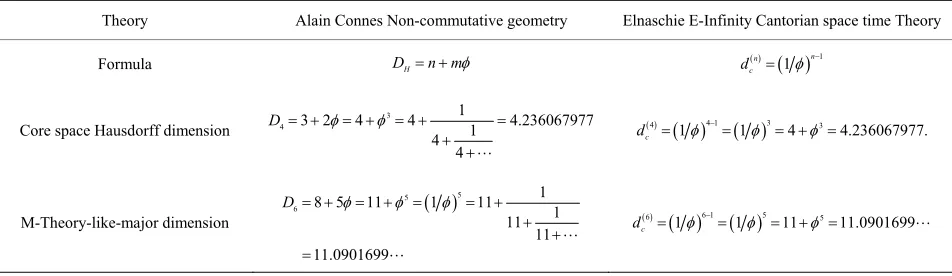
classical space time. A comparison reflecting the equiva- lence between A. Connes’ non-commutative geometry and E-Infinity Theory is given in Table 2.

7. Conclusions

First we presented a unified Newtonian-relativistic- quantum formula for quantum relativistic energy [20]. The homology of K3 Kähler and what we may call extra “dark” dimensions is the definite cause behind the sup- posedly missing dark energy [4,19]. To arrive at the cor- rect quantitative result and reconcile theory with experi- ments and cosmological measurements we need to scale the classical _{E mc} 2 by a scale relativity factor

QR

 defined as the ratio of two second Betti numbers [10,11]. Since the Betti number of fuzzy Kähler ₂ is 22 + k and since 2 for Einstein space of special Relativity, our

b

1 b 

QR

 becomes equal to 1 22



k



and one finds



b



 

_mc2

2 1 [9]. This means the missing dark en- ergy of the cosmos is exactly equal to

E b



1QR

 

100 

mc

95.4915028%. It is almost a dream world how the results of cosmic measurement are close to this percentage [4]. Noting that 2 may also be written as

QR QR

E 

5 ₂

 which means half of Hardy’s quantum entangle- ment probability found using orthodox quantum me- chanics and confirmed through sophisticated quantum information experiments [16,17,22], we feel that the or- dinary sharp non-fuzzy K3 Kähler manifold approxi- mates quantum gravity space time geometry and topol- ogy to an astonishing extent and must be real. Seen that way, we must infer that the Creator is a mathematician [1] with a deep inclination towards topology, geometry and number theory [7]. From a purely intuitive view point however the result is not surprising when we remember that in terms of particle physics Einstein’s special relativ- ity could in principle be found from a Lagrange with a single generalized coordinate, namely the photon [24-26]. A realistic theory of nature however must have a La- grangian with a minimum of 12 generalized coordinates

representing 12 massless gauge Bosons being the number of messenger particles of the standard model of high en- ergy physics [1,7,14]. The fundamental similarity factor found here 1 22 is mathematically the Lagrangian multiplier of an Isoperimetric variational problem when setting _mc2_{1 [30,31] and physically is the effect of}

quantum entanglement of the Hardy type on relativity for a single particle _5 _{2 i.e. where }5 _{1 11 for two par-}

ticle entanglement [22]. We checked our result using at least 24 different theories including Nottale’s scale rela- tivity [3,25] Magueijo and Smolin’s varying speed of light theory [5,6], Witten’s M-theory [23], Veneziano’s dual resonance theory and quantum field Yang-Mills theory in curved space time [1] and obtained exactly the same robust result reported here (see Table 1). One

striking point in the above analysis is the basic funda- mental similarity of the energy equations of Newton, Einstein and quantum relativity. This can be explained as follows:

There is nothing more fundamental and abstract like the notion of energy [1]. That is why self similarity mani- fests itself here directly as simple scaling from Newton to Einstein and beyond all that, to quantum gravity [1,3,5,6, 12,15]. This point is taken few steps further in Table 3.

This self-similarity or self-affinity is an important engi- neering concept in testing for instance Tsunami waves in small hydrodynamics laboratories [32]. It is also what made E. Witten discover that all the 5 different super- string theories are different facets of one theory [1,23]. Self-similarity exists in nature at all levels in the form of fractals [2,5]. Finally summing over all these self-similar objects and dimensions gives us a probabilistic constant value for the experimental speed of light exactly as it gave us the expectation value of the topological and Hausdorff dimension of spacetime namely DT = 4 and

. Ontologically the speed of light varies from Zero to Infinity however in DT = 4, it is a

constant expectation value and we should have suspected long ago that this alone is the clearest manifestation of

3

4 4.23606

H

[image:10.595.60.536.584.722.2]

D   

Table 2. The equivalence between non-commutative geometry and E-infinity formalism.

Theory Alain Connes Non-commutative geometry Elnaschie E-Infinity Cantorian space time Theory

Formula DH n m    

1

1 n

n c

d  



Core space Hausdorff dimension

3 4

1

3 2 4 4 4.236067977

1 4

4

D       



 4 _{ 1} 4 1 _{ 1} 3 ₄ 3 _4.236067977.

c

d    

    

M-Theory-like-major dimension  

5 5 6

1

8 5 11 1 11 ₁

11 11 11.0901699

D         



  

 6 _{ 1} 6 1 _{ 1} 5 ₁₁ 5 _11.0901699

c

d    

     

P.S.: 5 _{is Hardy’s probability of quantum entanglement and corresponds to negative topological dimension 4}

T

[image:11.595.53.537.100.200.2]

Table 3. Fundamental theories.

Topological Dimension (Menger-Uhryson) Formula Normalized

Classical mechanics 3 Positive topological dimensions 1 2

2

E mv 1

2

E

Special relativity 4 Positive topological dimensions _{E mc} 2 _E1

Hardy’s quantum entanglement probability −4 Negative Menger-Urhyson topological dimensions _P_Hardy_5 _E5

Immirzi quantum entanglement probability −5 Negative Menger-Urhyson topological dimensions _P_Immirzi_6 _E6

Note that in view of the above, Hardy’s entanglement represents a normalization of energy which is twice as large as the energy of a single particle according to

the quantum relativity theory presented here with  5₂

QR

[image:11.595.58.537.256.385.2]

E   _mc2 _where  _{2 1}



_{ 5}



.

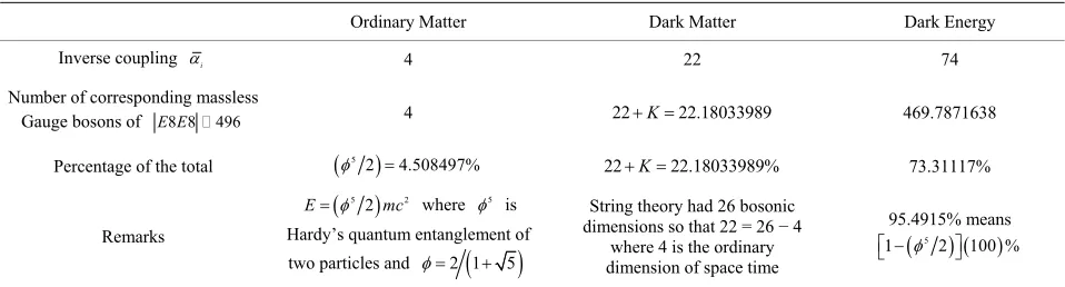
Table 4. Quantitative comparison between ordinary matter, dark matter and dark energy.

Ordinary Matter Dark Matter Dark Energy

Inverse coupling i 4 22 74

Number of corresponding massless

Gauge bosons of E E8 8 496 4 22 K 22.18033989 469.7871638

Percentage of the total



_5 ₂



_4.508497%

22 K 22.18033989% 73.31117%

Remarks



5 ₂



E  _mc2 _{where }5 _is

Hardy’s quantum entanglement of two particles and 2 1



 5



String theory had 26 bosonic dimensions so that 22 = 26 − 4

where 4 is the ordinary dimension of space time

95.4915% means



5



 

1  2 100

  

  %

P.S.: One may loosely say dark energy to mean the sum of both dark matter (22.18033%) and dark energy (73.31117%) so that the total is 95.4915%.

the fractality of our real quantum space time [17,29]. In

Table 4 we conclude by distinguishing between dark en-

ergy and dark matter and give the final results and per- centages with hints about the method of analysis.

REFERENCES

[1] R. Penrose, “The Road to Reality,” Jonathan Cape, Lon- don, 2004.

[2] Y. Baryshev and P. Teerikorpi, “Discovery of Cosmic Fractals,” World Scientific, Singapore, 2002.

[3] L. Nottale, “Scale Relativity,” Imperial College Press, London, 2011.

[4] L. Amendola and S. Tsujikawa, “Dark Energy: Theory and Observations,” Cambridge University Press, Cam- bridge, 2010.

[5] J. Mageuijo and L. Smolin, “Lorentz Invariance with an Invariant Energy Scale,” 18 December 2001, arXiv:hep- th/0112090V2.

[6] J. Mageuijo, “Faster Than the Speed of Light,” William Heinemann, London, 2003.

[7] M. S. El Naschie, “The theory of Cantorian Spacetime and High Energy Particle Physics (an Informal Review),” Chaos, Solitons & Fractals, Vol. 41, No. 5, 2009, pp. 2635-2646. doi:10.1016/j.chaos.2008.09.059

[8] M. S. El Naschie, “The Discrete Charm of Certain Eleven Dimensional Spacetime Theory,” International Journal of Nonlinear Sciences and Numerical Simulation, Vol. 7, No.

4, 2006, pp. 477-481.

[9] C. Nash and S. Sen, “Topology and Geometry for Phy- sicists,” Academic Press, San Diego, 1983.

[10] D. Joyce, “Compact Manifolds with Special Holonomy,” Oxford Press, Oxford, 2003.

[11] S. Yau and S. Nadis, “The Shape of Inner Space,” Perseus Book Group, New York, 2010.

[12] J. Polchinski, “String Theory,” Cambridge University Press, Cambridge, 1999.

[13] M. S. El Naschie, “On a Class of Fuzzy Kähler-Like Manifolds,” Chaos, Solitons & Fractals, Vol. 26, No. 2, 2005, pp. 257-261. doi:10.1016/j.chaos.2004.12.024 [14] M. S. El Naschie, “E-Infinity—Some Recent Results and

New Interpretations,” Chaos, Solitons & Fractals, Vol. 29, No. 4, 2006, pp. 845-853.

doi:10.1016/j.chaos.2006.01.073

[15] C. Rovelli, “Quantum Gravity,” Cambridge Press, Cam- bridge, 2004. doi:10.1017/CBO9780511755804

[16] M. S. El Naschie, “Quantum Entanglement as a Conse- quence of a Cantorian Micro Spacetime Geometry,” Journal of Quantum Information Science, Vol. 1, 2011, pp. 50-53. doi:10.4236/jqis.2011.12007

http://www.SCRIP.org/journal/jqis

[17] J.-H. He, et al., “Quantum Golden Mean Entanglement Test as the Signature of the Fractality of Micro Space- time,” Nonlinear Science Letters B, Vol. 1, No. 2, 2011, pp. 45-50.

http://en.wikipedia.org/wiki/Planck

[19] R. Panek, “Dark Energy: The Biggest Mystery in the Uni- verse,” The Smithsonian Magazine, 2010.

http://www.smithsonianmagazine.com/science-nature/Dar k-Energy

[20] D. R. Finkelstein, “Quantum Relativity,” Springer, Berlin, 1996. doi:10.1007/978-3-642-60936-7

[21] H. Saller, “Operational Quantum Theory,” Springer, Ber- lin, 2006.

[22] L. Hardy, “Non-Locality of Two Particles without In- equalities for Almost All Entangled States,” Physical Re- view Letters, Vol. 71, No. 11, 1993, pp. 1665-1668. doi:10.1103/PhysRevLett.71.1665

[23] M. Duff, “The World in Eleven Dimensions,” IOP Pub- lishing, Bristol, 1999.

[24] M. S. El Naschie, “Revising Einstein’s E = mc2_{. A The-} oretical resolution of the Mystery of Dark Energy,” Con- ference Program and Abstracts of the Fourth Arab In- ternational Conference in Physics and Material Sciences, Alexandria, 1-3 October 2012, p. 1.

[25] M. S. El Naschie and L. Marek-Crnjac, “Deriving the Ex- act Percentage of Dark Energy Using a Transfinite Ver-

sion of Nottale’s Scale Relativity,” International Journal of Modern Nonlinear Theory and Application, in Press, 2012.

[26] J.-H. He, “A Historical Scientific Finding on Dark En- ergy,” Fractal Spacetime and Non-Commutatitve Geome-try in Quantum and High Energy Physics, Vol. 2, No. 2, 2012. p. 154.

[27] L. Sigalotti and A. Mejias, “The Golden Mean in Special Relativity,” Chaos, Solitons & Fractals, Vol. 30, No. 3, 2006, pp. 521-524. doi:10.1016/j.chaos.2006.03.005 [28] S. Hendi and M. Sharif Zadeh, “Special Relativity and the

Golden Mean,” Journal of Theoretical Physics, Vol. 1, IAU Publishing, 2012, pp. 37-45.

[29] L. Smolin, “Three Roads to Quantum Gravity,” Wein- denfald & Nicolson, London, 2000.

[30] M. S. El Naschie, “Stress, Stability and Chaos in Struc- tural Engineering,” McGraw Hill, London, 1990. [31] C. Lanczos, “The Variational Principles of Mechanics,”

4th Edition, University of Toronto Press, Toronto, 1949. [32] G. Barenblatt, “Scaling,” Cambridge University Press,