SMOS-derived thin sea ice thickness: algorithm baseline, product specifications and initial verification

www.the-cryosphere.net/8/997/2014/ doi:10.5194/tc-8-997-2014

© Author(s) 2014. CC Attribution 3.0 License.

SMOS-derived thin sea ice thickness: algorithm baseline, product

specifications and initial verification

X. Tian-Kunze1, L. Kaleschke1, N. Maaß1, M. Mäkynen2, N. Serra1, M. Drusch3, and T. Krumpen4 1_{Institute of Oceanography, University of Hamburg, Bundesstraße 53, 20146 Hamburg, Germany}

2_{Finnish Meteorological Institute, Erik Palmenin aukio 1, 00560 Helsinki, Finland} 3_{European Space Agency, ESA-ESTEC, 2200 AG Noordwijk, the Netherlands}

4_{Alfred Wegener Institute for Polar and Marine Research, Bussestraße 24, 27570 Bremerhaven, Germany}

Correspondence to: X. Tian-Kunze ([email protected])

Received: 21 November 2013 – Published in The Cryosphere Discuss.: 6 December 2013 Revised: 4 April 2014 – Accepted: 10 April 2014 – Published: 27 May 2014

Abstract. Following the launch of ESA’s Soil Moisture and Ocean Salinity (SMOS) mission, it has been shown that brightness temperatures at a low microwave frequency of 1.4 GHz (L-band) are sensitive to sea ice properties. In the first demonstration study, sea ice thickness up to 50 cm has been derived using a semi-empirical algorithm with constant tie-points. Here, we introduce a novel iterative retrieval algo-rithm that is based on a thermodynamic sea ice model and a three-layer radiative transfer model, which explicitly takes variations of ice temperature and ice salinity into account. In addition, ice thickness variations within the SMOS spa-tial resolution are considered through a statistical thickness distribution function derived from high-resolution ice thick-ness measurements from NASA’s Operation IceBridge cam-paign. This new algorithm has been used for the continuous operational production of a SMOS-based sea ice thickness data set from 2010 on. The data set is compared to and vali-dated with estimates from assimilation systems, remote sens-ing data, and airborne electromagnetic soundsens-ing data. The comparisons show that the new retrieval algorithm has a con-siderably better agreement with the validation data and de-livers a more realistic Arctic-wide ice thickness distribution than the algorithm used in the previous study (Kaleschke et al., 2012).

1 Introduction

Satellite-based observation of ice thickness is still very chal-lenging. The first satellite-borne observations of ice thick-ness were conducted with satellite radar altimeters carried on European Remote Sensing satellites (1 and ERS-2) (Laxon et al., 2003) and thermal imagery from the Ad-vanced Very High Resolution Radiometer (AVHRR) (Yu and Rothrock, 1996; Drucker et al., 2003). These early radar altimeter observations were followed by the ICESat laser altimeter from 2003 to 2009 (Kwok and Cunning-ham, 2008) and, since 2011, by the CryoSat-2 radar al-timeter (Laxon et al., 2013). The radar and laser altime-ters have large uncertainties for ice thickness less than 1 m (Laxon et al., 2003; Kwok and Cunningham, 2008). There-fore, they are more suitable for the detection of thick ice. The altimeter ice thickness charts typically have a one month temporal resolution and a 25–100 km spatial resolution.

thin sea ice is needed. Since in situ measurements of snow thickness are seriously lacking in the Arctic, snow thickness from climatology (Warren et al., 1999) or from a thermody-namic sea ice model forced with numerical weather predic-tion model data (Launiainen and Cheng, 1998) can be used. Typically, snow thickness uncertainty is one of the main fac-tors determining the uncertainty of the retrieved ice thickness (Yu and Rothrock, 1996; Wang et al., 2010).

Passive microwave radiometer data from the Special Sen-sor Microwave Imager (SSM/I) (37 and 85.5 GHz channels) and Advanced Microwave Scanning Radiometer-Earth Ob-serving System (AMSR-E) (36.5 and 89 GHz channels) sen-sors have been used to estimate the thickness of thin ice to 10–20 cm (Martin et al., 2005; Tamura et al., 2007; Ni-hashi et al., 2009; Tamura and Ohshima, 2011; Singh et al., 2011). The spatial resolution of the radiometer-based thin ice thickness charts (6.25 to 25 km) is much coarser than that from thermal imagery, but daily Arctic and Antarctic cov-erage is possible. The thin ice thickness retrieval algorithms are linear or exponential regression equations between polar-ization ratios (PR) or the V- to H-polarpolar-ization ratios (R) and AVHRR or Moderate Resolution Imaging Spectroradiome-ter (MODIS) thicknesses. Naoki et al. (2008) suggested that the observed decrease of near ice surface salinity as a func-tion of ice thickness, which results in the modificafunc-tion of the ice dielectric properties and further ice emission (i.e., bright-ness temperatures), is the main reason for the observed re-lationship between brightness temperature and ice thickness. In addition, the relationship between brightness temperature and ice thickness is more pronounced for H-polarization and for a lower frequency (e.g., 10.7 GHz). Nihashi et al. (2009) found that PR at 37 GHz cannot detect thin ice when it is cov-ered with snow. An analysis of ship-borne radiometer data at 19, 37, and 85 GHz over various thin ice types indicated that a limitation in the thin ice thickness estimation can be attributed to the presence of snow or dense frost flower cov-erage (>60 %) on the ice surface (Hwang et al., 2007).

The Soil Moisture and Ocean Salinity (SMOS) mission of the European Space Agency (ESA) was launched in Novem-ber 2009, and for the first time, globally measures Earth’s radiation at a frequency of 1.4 GHz in the L-band (Mecklen-burg et al., 2012). The spatial resolution varies from about 35 km to more than 50 km. Besides soil moisture and ocean salinity information, for which SMOS was originally de-signed, L-band radiometry on SMOS can also be used to obtain sea ice thickness, which is due to its large penetration depth in sea ice (Kaleschke et al., 2010, 2012). The measured L-band brightness temperature mainly depends on the ice concentration, the molecular temperatures of the sea and the ice, and their emissivities (Menashi et al., 1993; Kaleschke et al., 2010). Sea ice emissivity depends on the microphysi-cal sea ice structure, but inhomogeneities, like brine pockets and air bubbles, are much smaller than the SMOS wavelength of 21 cm (Kaleschke et al., 2010, 2012). Therefore, we can consider sea ice as a homogeneous medium and ignore

vol-ume scattering. The modeled sea ice emissivity used for the present study mainly depends on ice thickness, ice tempera-ture, and ice salinity (Kaleschke et al., 2010).

In contrast to ICESat and CryoSat-2 measurements, SMOS-derived ice thickness has a lower uncertainty in the thin ice range, but an exponentially increasing uncertainty for ice thickness thicker than 0.5 m. In our study, we con-sider ice thickness less than 50 cm as thin ice. SMOS-derived ice thickness can thus complement the measurements from CryoSat-2 to achieve Arctic-wide sea ice thickness estima-tions (Kaleschke et al., 2010, 2012).

The semi-empirical SMOS ice thickness retrieval algo-rithm applied previously in Kaleschke et al. (2012) (here-inafter Algorithm I) is

TB(dice)=T1−(T1−T0)e−γ dice, (1) wheredice is the ice thickness,T1 andT0are two constant tie points, which were estimated from the observed SMOS brightness temperatures over open water and thick first year ice during the freezing period of 2010 in the Arctic, andγ is a constant attenuation factor, which was derived from a sea ice radiation model (Menashi et al., 1993) for a representative bulk ice temperature and salinity in the Arctic.

The advantage of Algorithm I is the retrieval of ice thick-ness from the brightthick-ness temperature (TB) without any aux-iliary data set. However, the TB measured by an L-band ra-diometer over sea ice depends on the dielectric properties of sea ice, which are functions of ice temperature and ice salinity (Kaleschke et al., 2010). Although the change of TB caused by the sea ice thickness variation is much larger than that caused by the variation of ice temperature and ice salin-ity, the typical variability of these two parameters in the Arc-tic can induce up to 30 K difference in TB (Kaleschke et al., 2012). This means, the assumption of constant retrieval pa-rameters could cause considerable errors in regions where these parameters strongly differ from the assumed constant values.

temperature from atmospheric reanalysis data as a boundary condition. Ice salinity can be estimated from the underlying sea surface salinity (SSS) with an empirical function (Ryvlin, 1974). With these two parameters, we can calculate bright-ness temperature with the sea ice radiation model (Menashi et al., 1993). However, both ice temperature and ice salinity are, in turn, functions of ice thickness. Thus, we need to ap-ply a linear approximation method to simultaneously retrieve ice thickness and estimate suitable ice temperature and salin-ity values. This algorithm is called Algorithm II hereinafter.

In the radiation model of Menashi et al. (1993), a plane ice layer is assumed. However, natural sea ice exhibits a sta-tistical thickness distribution within the spatial resolution of SMOS, due to dynamic-thermodynamic growth and defor-mation processes (Bartels-Rausch et al., 2012). The ness temperature measured by SMOS is a mixture of bright-ness temperatures from different ice thickbright-nesses, and possi-bly open water. As SMOS brightness temperature is more sensitive to ice thicknesses less than 0.5 m (Kaleschke et al., 2012), SMOS-derived ice thickness depends on the thin ice part of the ice thickness distribution within the spatial reso-lution, while the contribution of the thicker ice part cannot be quantified due to the limited penetration depth. Thus, the overall mean thickness for a mixture of thin and thick ice can only be estimated in a statistical sense if the thickness distribution function is known. A possible solution for the corresponding underestimation of ice thickness is to correct the retrieved ice thickness, using an ice thickness distribution function. The correction of ice thickness retrieved from Al-gorithm II using this function is called AlAl-gorithm II* in this study.

Here, we compare the three different SMOS ice thickness retrieval algorithms for the Arctic. The plane layer ice thick-nesses retrieved from Algorithm I and II are compared with independent data to examine if the method that considers variable ice temperature and ice salinity improves the accu-racy of the ice thickness retrieval. Thereafter, sea ice thick-ness uncertainty is estimated on a daily basis, using the better algorithm. The growth of the sea ice cover, as seen by SMOS during a freezing period in the Arctic, is also discussed.

The paper is structured as follows. In Sect. 2, we de-scribe the SMOS brightness temperature and the auxiliary data sets. The baseline of Algorithm II is described in Sect. 3. In Sect. 4, we discuss the uncertainties and biases of the re-trieved ice thickness. After that we present, in Sect. 5, our method to correct the retrieved ice thickness based on the as-sumption of a plane ice layer with an empirically determined ice thickness distribution function. The comparison of ice thicknesses retrieved from different algorithms is discussed in Sect. 6. Ice thickness growth and distribution, as seen by SMOS during the freeze-up period in the Arctic are shown in Sect. 7. A further comparison of SMOS-derived ice thickness with that derived from MODIS in the Kara Sea is presented in Sect. 8. Finally, a summary and discussion are given in Sect. 9.

2 Data

Three different data sets are used for the retrieval of sea ice thickness in Algorithm II. The basis of the retrieval is the brightness temperature measured by the SMOS L-band ra-diometer. This data set is described in Sect. 2.1. For the esti-mation of bulk ice temperature (Tice) we use surface air tem-perature (Ta) from Japanese 25 yr Reanalysis (JRA-25) data, which are described in Sect. 2.2. The SSS climatology, which is used for the calculation of bulk ice salinity (Sice) is pre-sented in Sect. 2.3. Finally, for the verification of the SMOS ice thickness, MODIS ice thickness charts over the Kara Sea are presented in Sect. 2.4.

2.1 SMOS brightness temperature data 2.1.1 L1C data

The SMOS payload Microwave Imaging Radiometer using Aperture Synthesis (MIRAS) measures in the L-band bright-ness temperatures in full polarization, with incidence angles ranging from 0◦to 65◦. All four Stokes parameters are ob-tained (Kerr et al., 2001). It has global coverage every three days (Kerr et al., 2001), whereas daily coverage up to 85◦ lat-itude can be expected in the polar regions. Brightness temper-ature is taken every 1.2 s by hexagon-like, two-dimensional snapshots, which have a spatial dimension of about 1200 km across (Kerr et al., 2001). The geometric distribution of inci-dence angles and radiometric accuracy within the alias-free areas of a snapshot (Camps et al., 2005) is shown in Fig. 1. The spatial resolution varies from about 35 km at nadir view to more than 50 km at incidence angles higher than 60◦_{. Each}

snapshot measures one or two of the Stokes components in the antenna reference frame. Horizontally and vertically polarized brightness temperatures are measured by separate snapshots.

The SMOS L1C data are geolocated in an equal-area Dis-crete Global Grid (DGG) system called ISEA 4H9 (Icosahe-dral Snyder Equal Area projection with aperture 4, resolution 9 and shape of cells as hexagon) (Pinori et al., 2008). ISEA 4H9 provides a uniform inter-cell distance of 15 km. Most of the pixels in the Arctic are covered by several overflights dur-ing one day. Therefore, for our daily product, at each DGG grid point we collect all brightness temperatures measured during one day, together with other information, like the in-cidence angles.

2.1.2 Radio frequency interference

0 20 40 60 80 100 120 140 0

50 100 150

10

20

30

40

50

60

3.0 3.5 4.0 4.5 5.0 5.5 6.0 6.5 7.0

Radiometr

ic

accur

acy

[K]

Figure 1. Distribution of radiometric accuracy within a typical

snapshot with incidence angles (degrees) as contour lines. To avoid the patchy distribution of DGG pixels within one snapshot, we over-laid 100 consecutive snapshots after axis transformation. After that, the radiometric accuracy and incidence angles are interpolated with 10 km spatial grid resolution.

(Camps et al., 2010). A closer look into RFI-contaminated snapshots shows that RFI can either completely or partly de-stroy a snapshot (Camps et al., 2010). For simplification, we apply a threshold value for both horizontally and ver-tically polarized brightness temperatures. If either of them exceeds 300 K within one snapshot, this snapshot is consid-ered RFI contaminated. Brightness temperatures higher than 300 K can not be expected in the Arctic and Antarctic.

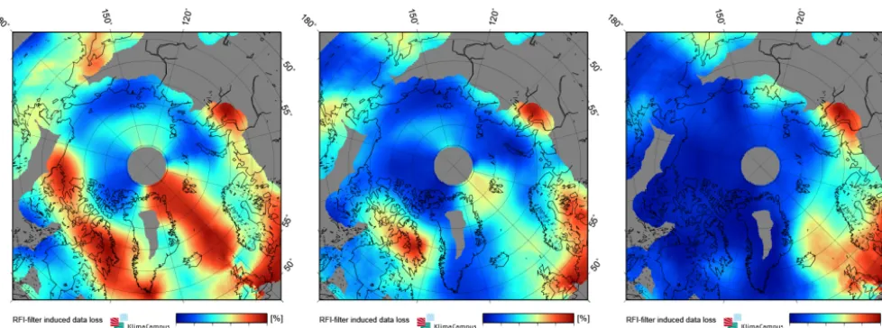
According to this RFI filter, strongly RFI-affected regions are the region northeast of Greenland and parts of the Cana-dian Arctic Archipelago. Figure 2 shows the RFI-induced data loss based on our RFI filter. The data loss in the figure is defined as the ratio between the number of RFI-contaminated measurements and the number of total measurements. As can be seen from Fig. 2, the status of RFI in the Arctic region has improved much since 2010.

2.1.3 Brightness temperature intensity

Over sea ice, the first Stokes parameter (intensity) is almost independent of incidence angle in the incidence angle range of 0–40◦_{(Fig. 3). The intensity is the average of the}

horizon-tally and vertically polarized brightness temperatures, equal to 0.5(TBh+TBv). The intensity is independent of both geo-metric and Faraday rotations, and robust to instrumental and geophysical errors (Camps et al., 2005). We can avoid ad-ditional uncertainties caused by the transformation from the antenna reference frame to the Earth reference frame by us-ing the intensity. Since each snapshot measures either

hor-izontally or vertically polarized brightness temperature, we use consecutive snapshots with an acquisition time difference of less than 2.5 s to calculate the intensity. The advantage of using near-nadir measurements is the smaller footprint as-sociated with low incidence angles. Furthermore, by using the whole incidence angle range of 0–40◦we get more than 100 brightness temperature measurements per day for most of the DGG grid points in the Arctic; and by averaging over numerous measurements we can significantly reduce the un-certainty of the retrieval. However, by averaging all the mea-surements, we partly reduce the geophysical and temporal variability. The daily averaged brightness temperature inten-sities in the Arctic and in the Antarctic are interpolated with a nearest-neighbor algorithm and gridded into the National Snow and Ice Data Center (NSIDC) polar stereographic pro-jection with a grid resolution of 12.5 km (https://nsidc.org/ data/polar_stereo/ps_grids.html). We use this grid resolution because other products that we use as auxiliary data in the re-trieval are also given in this resolution. We call this product L3B brightness temperature. In the following we use TB to indicate the daily averaged brightness temperature intensity. The data are processed with about 24 h latency for both hemi-spheres, and cover a period since January 2010. The L3B TBs are the basis of our sea ice thickness retrieval with Al-gorithm I and II and can be obtained from icdc.zmaw.de. 2.2 JRA-25 reanalysis data

For estimating the ice surface temperature, we extract the 2 m surface air temperature and the 10 m wind velocity data from JRA-25 atmospheric reanalysis data and interpolate them into the polar stereographic projection with 12.5 km grid resolution. JRA-25 reanalysis data provide various physical variables with 1.125◦ resolution every six hours. The data have been produced by the Japanese Meteorological Agency (JMA) using the latest numerical analysis and prediction sys-tem. 25 covers the period from 1979 to 2004. JRA-25 has been transitioned to JMA Climate Data Assimilation System (JCDAS), which takes over JRA-25 after 2005 on a real-time basis using the same assimilation system (Onogi et al., 2007). Various studies have been carried out comparing the JRA-25, ERA40 and National Centers for Environmen-tal Prediction (NCEP) data sets. Good agreement was found between JRA-25 and ERA40 (Onogi et al., 2007).

2.3 Sea surface salinity climatology

Figure 2. The induced data loss in the Arctic from 2010 to 2012. The data loss is defined as the ratio between the number of

RFI-contaminated measurements and the number of total measurements. A strongly reduced data loss can be observed in 2012 especially in the Canadian Arctic Archipelago compared with the map of 2010.

0 10 20 30 40 50 60

Incidence angle Θ [◦]

180 190 200 210 220 230 240 250 260 270

Brightness temperature [K]

0.5(V+H)

V

H

Figure 3. Vertically (V) and horizontally (H) polarized TBs and the

first Stokes parameter as a function of incidence angle calculated using a three-layer model for sea ice with a thickness ofdice=1 m, a bulk salinity ofSice=8 g kg−1, and a bulk ice temperature of

Tice= −7◦C.

climatology based on the output of an ocean-sea ice coupled model.

The SSS data used in this work result from an integration of the MIT General Circulation Model (MITgcm) (Marshall et al., 1997), including interannually varying surface forc-ing. The model is configured for the Atlantic Ocean north of 33◦S, including all marginal Atlantic seas and the Arc-tic Ocean and with the Bering Strait as a boundary, and is integrated at the eddy-resolving resolution of approximately 4 km. The vertical resolution of the model varies from 5 m in the upper ocean to 275 m in the deep ocean (100

verti-cal levels are used). Bottom topography is interpolated from the ETOPO2 database (Smith and Sandwell, 1997) and ini-tial temperature and salinity conditions from a 8 km res-olution integration of the same model (to achieve a good degree of spin-up), which in turn were obtained from the WOA09 climatology (Locarnini et al., 2010; Antonov et al., 2010). The model is forced at the surface by fluxes of mo-mentum, heat, and freshwater, computed internally in the model with the help of the 6 hourly atmospheric state from the European Centre for Medium-Range Weather Forecasts ERA-Interim reanalysis (Dee et al., 2011) and bulk for-mula. At the open boundaries, the model is forced by a 1◦ resolution global solution. The K-Profile Parameterization (KPP) formulation is used for the parameterization of ver-tical mixing, with a background verver-tical viscosity coefficient of 1×10−4m2s−1. The vertical diffusion employed amounts to 1×10−5m2s−1. Unresolved horizontal mixing uses a bi-harmonic diffusion/viscosity of 3×109m4s−1. Annually av-eraged river run-off based on the Fekete et al. (1999) data set is introduced as a virtual salt flux, which is summed at certain coastal grid points (approximately the river mouths) to freshwater forcing, specifically to precipitation (from the ERA reanalysis) minus evaporation (computed in the model). The overall good performance of this model configuration (integrated at 8 km resolution), assessed through compar-isons with in situ measurements, can be found in Serra et al. (2010); Brath et al. (2010); Dmitrenko et al. (2012).

20 25 30 35 40 [gkg-1_]

0 1 2 3 4

[gkg-1_]

Fig. 4.Mean and standard deviation of weekly sea surface salinity for the winter period from October to

April, based on 8yrof daily model output.

43

Figure 4. Mean (left map) and standard deviation (right map) of weekly sea surface salinity for the winter period from October to April,

based on 8 yr of daily model output.

“weekly climatology”. We choose to use a model climatol-ogy and not the Polar Science Center Hydrographic Clima-tology (PHC) (Steele et al., 2001) in order to benefit from the dynamical oceanographic structures realistically resolved in the model, which leads to spatial and seasonal variability of SSS.

Figure 4 shows the mean and standard deviation of weekly SSS from October to April, based on the 8 yr of daily model output. SSS in the Laptev Sea, parts of the Kara Sea, and the Baltic Sea is much lower than that in the central Arctic due to the influence of river run-offs. In contrast, in Baffin Bay, the Greenland Sea, and the Barents Sea, SSS is higher than in the central Arctic. The mean weekly SSS in the Baltic sea varies in the range of 4–10 g kg−1, which agrees well with the observed climatology given in Janssen et al. (1999). To calculate Arctic-wide ice thickness distributions, it is impor-tant to use the spatially and temporally variable weekly SSS climatology.

2.4 MODIS ice thickness charts

MODIS ice thickness charts have been calculated covering an area of 1500 km×1350 km over the Kara Sea and the east-ern part of the Barents Sea. The derivation of the charts and their uncertainty estimation are described in detail in Maeky-nen et al. (2013). The total number of charts is 120, and they cover two winters (November to April) in 2009–2011. The spatial resolution of the charts is 1 km, and they show ice thickness from 0 to 99 cm. The external forcing data for solv-ing the ice thickness from the surface heat balance equation come from the numerical weather prediction (NWP) model HIRLAM (HIgh-Resolution Limited Area Model) (Kaellen, 1996; Unden, 2002). Only nighttime MODIS data are em-ployed. Thus, the uncertainties related to the effects of solar

shortwave radiation and surface albedo are excluded. For the cloud masking of the MODIS data, in addition to the different cloud tests (Frey et al., 2008), manual methods are also used in order to improve the detection of thin clouds and ice fog. The cloud masking is conducted with 10 km×10 km blocks to identify larger cloud-free areas and to reduce errors due to the MODIS-sensor striping effect. In the ice thickness chart calculation, an average snow thickness (hs) to ice thickness (hi) ratio is used. The thickness of the snow layer is assumed to be

hs=0 m for dice<0.05 m,

hs=0.05×dice for 0.05 m≤dice<0.2 m,

hs=0.09×dice for dice≥0.2 m.

This relationship is based on Doronin (1971) and the So-viet Union’s Sever expeditions data (NSIDC, 2004). The typ-ical maximum reliable ice thickness (max 50 % uncertainty) is estimated to be 35–50 cm under typical weather conditions (air temperatureTa<−20◦C, wind speedVa<5 ms−1) for

3 Sea ice thickness retrieval Algorithm II

Algorithm I is described in detail in Kaleschke et al. (2012). We will here introduce the retrieval Algorithm II. As in Al-gorithm I, we use the daily mean brightness temperature in-tensity TB averaged over 0–40◦incidence angle range. 3.1 The sea ice radiation model

The basis of the SMOS ice thickness retrievals Algorithm I and II is the sea ice radiation model adapted from Menashi et al. (1993). While for Algorithm I the radiation model is used to calculate the constant attenuation factorγ for a rep-resentative Tice and Sice in the Arctic, in Algorithm II the model is used to calculate TB at variableTiceandSice.

The sea ice radiation model consists of a plane ice layer bordered by the underlying sea water and air on the top. The model does not allow adding a snow layer. A snow layer has a twofold effect on the L-band emission. One is the thermo-dynamic insulation effect, which will be discussed in the fol-lowing section, the other is the radiative contribution to the overall brightness temperature. To consider the second effect, an elaborate inter-comparison with a multi-layer emission model that includes a snow layer (e.g., Maaß et al., 2013b) would be necessary. The TB over sea ice depends on the di-electric properties of the ice layer, which are a function of brine volume (Vant et al., 1978). The brine volume is a func-tion ofSiceandTice(Cox and Weeks, 1983).

For a thin ice layer, the ice temperature gradient within the ice can be assumed to be linear (Maaß, 2013a). Assuming that the water under sea ice is at the freezing point, we can calculate Tice with 0.5(Tsi+Tw), whereTsi is the snow-ice interface temperature, andTw is the freezing sea water tem-perature. TheTsiis calculated with a thermodynamic model withTaas a boundary condition. The thermodynamic model is presented in the next section.

Sice is estimated using the empirical function of Ryvlin (1974):

Sice=Sw(1−SR)e−a

√ dice_+S

RSw, (2)

whereSwis the SSS,diceis the ice thickness (here in cm),SR is the salinity ratio of the bulk ice salinity at the end of the ice growth season, and the SSS,ais the growth rate coefficient, which varies from 0.35 to 0.5. Ryvlin (1974) suggests using 0.5 foraand 0.13 forSR. However, Kovacs (1996) compares the Ryvlin empirical equation with observed data in the Arc-tic and suggests using 0.175 forSR instead of 0.13. In our model, we use 0.175 forSR, which seems to fit better to the observation data of ice salinity in the Arctic. Cox and Weeks (1983) give another empirical relationship betweenSiceand dice in the Central Arctic. The two empirical relationships have similar values for first year ice and a water salinity of

Sw=31 g kg−1(Kovacs, 1996). TheSicein Eq. (2) is a func-tion of the underlying SSS. Therefore, we can calculate ice salinity based on the Arctic-wide SSS climatology.

0.0 0.2 0.4 0.6 0.8 1.0

Ice thickness [m]

100 120 140 160 180 200 220 240 260

Brightness temperature [K]

Tice

= -20

Tice

= -10

Tice

= -5

Tice

= -2

dmax

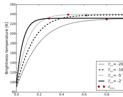
Figure 5. TB as function ofdiceunder differentTice, calculated with the sea ice radiation model with aSiceof 8 g kg−1

The ice thickness retrieval with SMOS data is limited by the saturation of TB. We consider TB to reach saturation if the change of TB withdiceis less than 0.1 K per cm. Thus, TB of an ice layer with aTiceof−2◦C and a salinity of 8 g kg−1 reaches its saturation for ice thicknesses of less than 30 cm, for example. This means that the maximal retrievable ice thicknessdmaxunder warm and saline conditions can be as low as a few centimeters. In contrast, under cold conditions and a low ice salinity, which is typical for coastal regions with river run-off, L-band TB emanates from a thicker ice layer. TB reaches its saturation much more slowly, anddmax can be as high as 1.5 m (Figs. 5 and 6). Therefore, SMOS ice thickness retrieval is more suitable for cold conditions and low ice salinity. If the ice temperature varies between−5◦_C

and−10◦_{C, which can be expected in thin-ice covered areas}

in the Arctic during the freeze-up period (Perovich and Elder, 2001), the difference of retrieved ice thicknesses can be as high as 20 cm. The influence of ice salinity on the ice thick-ness retrieval increases with decreasing ice salinity (Maaß, 2013a). For example, under aTice of −10◦C, the dmax at 1 g kg−1Sicecan be twice of that at 5 g kg−1Sice.

3.2 The thermodynamic model

−20 −15 −10 −5 0

Bulk ice temperature [◦_C] 0.0

0.5 1.0 1.5 2.0 2.5

Maximal

retr

ie

vab

le

ice

thic

kness

[m]

Sice=1 Sice=5 Sice=10 Sice=15

Figure 6.dmaxunder differentTice[◦C] andSice[g kg−1].

and snow layers in the model. The snow thicknesshsis calcu-lated withdiceaccording to the relationship given in Doronin (1971) (see Sect. 2.4).

Under the assumption of thermal equilibrium, the incom-ing and outgoincom-ing heat fluxes compensate each other. Durincom-ing winter season, surface melting can be ignored. Therefore, the heat balance at the surface of a slab ice layer with thickness

diceand a layer of snow with thicknesshson top can be de-scribed as

(1−α)Fr−I0+FLin−FLout+Fs+Fe+Fc=0, (3) whereFris the incoming shortwave radiation,αis the albedo of the snow/ice layer,I0is the part of the incoming shortwave radiation that is transmitted into the ice,FLinis the incoming longwave radiation, FLout is the outgoing longwave radia-tion, Fs is the sensible heat flux,Fe is the latent heat flux, andFcis the conductive heat flux.

The radiative and turbulent fluxes (1−α)Fr−I0, FLin, FLout, Fe, and Fs are calculated as in Maykut (1986). For simplification we assume constant values for the cloud cover

C, the relative humidityr, and the bulk transfer coefficients for sensible and latent heat fluxCsandCeestimated from the reanalysis data. However, these parameters can be obtained from the auxiliary data that will be delivered with SMOS L1C data in the future.

The conductive heat fluxFcis given by

Fc=

kiks kihs+ksdice

(Tw−Ts), (4)

whereks andki are the thermal conductivities of snow and ice,Twis the freezing point of sea water, andTsis the snow surface temperature. In the case of bare ice,Tsis the ice sur-face temperature.ks is set to 0.31 W m−1K−1according to Yu and Rothrock (1996). The thermal conductivity of iceki

can be expressed as (Untersteiner, 1964)

ki=2.034+0.13 Sice Tice−273

, (5)

whereSiceis in g kg−1andTiceis in K.Ticecan be calculated with

Tice=0.5(Tsi+Tw), (6)

whereTsi is the snow-ice interface temperature calculated with

Tsi=

Ts+_kk_si_dh_ices Tw

1+ kihs ksdice

. (7)

To calculateTsiwe need to knowki. However,ki is in turn a function ofTice. As an approximation, we first calculateki with 0.5(Ts+Tw)instead of 0.5(Tsi+Tw). Here we ignore the difference betweenTsandTsi. This makes a minimal change inki.Ts is estimated with least-square method for eachdice under the thermal equilibrium assumption.

3.3 Retrieval steps

As discussed in Sect. 3.1, the challenge of using variableTice andSicein Algorithm II is that both are functions ofdice. The algorithm is based on the forward model consisting of the ra-diation and thermodynamic models. Therefore, we approxi-matedice by iterating the radiation and the thermodynamic models until a convergence point is found for the solution (Fig. 7). In this process, at each stepTiceandSiceare calcu-lated for the respectivediceapproximation. The starting point of the iteration is thedice retrieved with Algorithm I, which uses a constantTice of−7◦C and Sice of 8 g kg−1. At each iteration step, we usedice,Tice, andSiceto calculate TB with the radiation model. The calculated TB is then compared with that observed by SMOS. To minimize the difference be-tween the observed and the calculated TBs, the newdiceis es-timated with a linear approximation method. We define two stopping criteria for the iteration, a brightness temperature difference of less than 0.1 K, or an ice thickness difference of less than 1 cm. The first criterion is defined by considering the radiometric accuracy of the brightness temperature mea-surements and the number of available daily meamea-surements. We apply the first criterion if the ice is thicker than 30 cm and otherwise we apply the second criterion. We determinedmax with the same criteria for the saturation of TB (the TB change is less than 0.1 K per 1 cmdice). We define a saturation factor

STB=dice/dmax. (8)

<>

Initial d from Algorithm I

d '=(TBobs−T0)

(TB−T₀)⋅d

TB TBobs

Tice=fT(d , Tair) Sice=fS(d , SSS)

TB=f_TB(d ,T_ice, S_ice)

Figure 7. Schematic flow chart of the retrieval steps.dandd0are the sea ice thicknesses from the consecutive steps, TB and TB_obs are calculated and observed brightness temperatures, andT0is the brightness temperature of sea water assumed to be 100.5 K.

This limitation can be identified if a grid point shows a low

dmaxand at the same time a high saturation ratio. Both pa-rameters are provided in our data set daily at each grid point.

4 Assessment of uncertainties 4.1 Systematic errors

In both algorithms we assume 100 % ice coverage for sim-plicity. TB over ice-sea water mixed areas can be described as

TB=TBwater×(1−IC)+TBice×IC, (9) where IC is the ice concentration, TBwaterand TBiceare the TBs over sea water and ice, respectively.

SMOS TBwatershows a stable value of about 100.5 K with a standard deviation of about 1 K in the Arctic region. With this constant TBwater, we can calculate TBice using ice con-centration charts from passive microwave radiometer data. During the winter, most of the ice covered area in the Arctic has ice concentrations (IC) higher than 90 % (Andersen et al., 2007). The passive microwave radiometer IC charts have an uncertainty of 5 % in the winter time (Andersen et al., 2007). At high concentrations, correcting the retrieved ice thickness with the IC data set with an uncertainty of 5 % can cause higher errors than the 100 % ice coverage assumption. There-fore, we assume 100 % ice coverage in the retrievals. The possible underestimation of ice thickness due to this

assump-20 30 40 50 60 70 80 90 100

Ice concentration [%]

0.0 0.1 0.2 0.3 0.4 0.5

Underestimation

of

ice

thic

kness

[m]

TB=140 K TB=160 K TB=180 K TB=220 K

Figure 8. The underestimation of ice thickness caused by the 100 %

ice coverage assumption.

tion is investigated with the simple semi-empirical function used in Algorithm I. Figure 8 shows that the bias caused by this assumption increases exponentially with decreasing ice concentration. If we assume a SMOS TB of 220 K, the bias can be very high even for IC of more than 80 %. At lower brightness temperatures, the bias caused by this assumption is less than a few centimeters.

4.2 Sea ice thickness uncertainties

There are several factors that cause uncertainties in the sea ice thickness retrieval: the uncertainty of the SMOS TB, the uncertainties of the auxiliary data sets, and the assumptions made for the radiation and thermodynamic models.

For our retrieval, we average TB over the incidence angle range of 0–40◦. There are usually more than 100 TB mea-surements per day at each grid point in the Arctic region. By averaging the measurements, we reduce the measurement un-certainty. We describe the variability of TB by dividing the standard deviation of TB with the square root of the number of measurements during one day at each grid point. The TB variability is usually lower than 0.5 K in the Arctic, except for the strongly RFI-affected regions. The uncertainties ofTice andSice depend on the uncertainties inTa and SSS, as well as the uncertainty caused by the missing physics. BothTaand SSS are derived from model outputs. Due to the sparse obser-vations in the polar regions,Taand SSS themselves contain large uncertainties.

difficult, because it depends not only onTa, but also on the assumptions made in the thermodynamic model. As a first approximation, we assume 1 K for the std(Tice), which is es-timated with the variations inTa. More investigations should be conducted to better estimate the uncertainty inTicein the future. The uncertainties provided in the current data set are first estimations. The different error factors are not indepen-dent, because they are functions of ice thickness. An elabo-rate investigation about the correlation between these error factors will be carried out. At present, each error caused by the standard deviations of brightness temperature, ice salin-ity, and ice temperature is estimated by keeping the other pa-rameters constant. The total uncertainty given in the data set is the sum of these errors. Errors caused by the assumptions about fluxes and snow thickness have not yet been included. We consider this as future work.

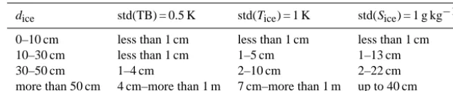
In Table 1, we show an example of estimated ice thickness uncertainties for conditions whereTicevaries from−10◦C to −2◦C, andSicevaries from 2 g kg−1to 8 g kg−1. We assume a standard deviation of 0.5 K, 1 K, and 1 g kg−1for TB,Tice, andSice, respectively. The ice thickness uncertainty caused by std(TB) is rather small for thin ice less than 50 cm, and in-creases exponentially for thicker ice. The uncertainty caused by std(Tice) is higher than that caused by std(TB), with an in-creasing trend with inin-creasing ice thickness. The uncertainty ofSicehas little impact on the ice thickness retrieval for saline ice withSiceof more than 5 g kg−1. However, for less saline ice, which is typical in regions with river run-off, std(Sice) has much more impact on the ice thickness uncertainty than the other two parameters whendiceis less than half a meter.

5 The effect of the subpixel-scale heterogeneity on the thickness retrieval (Algorithm II* post-processing) The limitations of SMOS measurements are twofold: (1) SMOS has a large spatial resolution (about 35 km at nadir view), and thus the SMOS signal comes from diverse ice types and even open water, within the resolution. It is difficult to decide what kind of ice thickness SMOS really measures, since the ice thickness distribution within the spatial reso-lution is not well known. (2) Under cold Arctic conditions, the maximum retrievable ice thickness from SMOS is about 50 cm, and varies depending on the ice temperature and ice salinity. SMOS-derived ice thickness depends on the thin ice part of the ice thickness distribution within the spatial reso-lution, while the contribution of the thicker ice part cannot be quantified due to the limited penetration depth. Thus, the overall mean thickness for a mixture of thin and thick ice can only be estimated in a statistical sense if the thickness distribution function is known.

Sea ice deformation patterns are often described using self-similar functions, such as the lognormal distribution (Er-lingsson, 1988; Key and McLaren, 1991; Tan et al., 2012). A theory of sea ice thickness distribution was developed by

Thorndike et al. (1975). Models that include ice growth and deformation may be used to simulate the evolution of the thickness distribution (Thorndike, 1992; Godlovitch et al., 2012). A common feature of simulations and empirical ob-servations is the exponential tail resulting from dynamic de-formation processes. The dominant effect of the thin ice part on the SMOS-derived ice thickness leads to a considerable underestimation of sea ice thickness if the retrieval model is based on a plane sea ice layer. In the following, we use airborne sea ice thickness measurements in order to param-eterize the thickness distribution function and to investigate the effect of the subpixel-scale heterogeneity on the thickness retrieval.

NASA’s Operation IceBridge (OIB) airborne campaigns obtained large scale profiles of sea ice thickness derived from a laser altimeter system (Kurtz et al., 2013). The footprint size of a single laser beam is about 1 m, and the vertical ac-curacy is given as 6.6 cm. The sea ice thickness is estimated from the freeboard by accounting for the snow thickness and by making assumptions about the densities of ice and snow. Simultaneously, the snow thickness is retrieved using a snow-depth radar. Here, we use the OIB “quicklook” data as ob-tained from the NSIDC website.

We assume that the sea ice thickness follows a lognormal distribution:

p(dice, µ, σ )= 1

diceσ √

2πe

−(log(dice)−µ) 2

(2σ2) _{, (10)}

with the two parameters logmeanµ and logsigma σ. Fur-thermore, we assume a constant logsigma valueσ to approx-imate the thickness distribution function with only one inde-pendent variable. To test this assumption, we split the 2012 and 2013 OIB Arctic sea ice thickness data into segments of about 30 km length. We found that using constant values

Table 1. Estimated ice thickness uncertainties caused by std(TB), std(Tice), and std(Sice).

dice std(TB) = 0.5 K std(Tice) = 1 K std(Sice) = 1 g kg−1

0–10 cm less than 1 cm less than 1 cm less than 1 cm 10–30 cm less than 1 cm 1–5 cm 1–13 cm

30–50 cm 1–4 cm 2–10 cm 2–22 cm

more than 50 cm 4 cm–more than 1 m 7 cm–more than 1 m up to 40 cm

superposition principle:

TB∗(dice)=

max(dice) Z

0

TB(dice)g(dice)ddice, (11)

with the thickness distribution function g(dice) and the brightness temperature of a single/plane-layer model TB(dice). While dmax is the maximum retrievable single-layer ice thickness, max(dice)is the maximum of ice thick-ness in the ice thickthick-ness distribution function. The bright-ness temperature weighted with the thickbright-ness distribution TB∗suggests a sensitivity to ice thicknesses larger thandmax. Here,dmaxanddiceboth refer to the single-layer thickness. The real mean thickness, denoted as H, is strongly under-estimated if the retrieval does not account for the thickness distribution. The overall effect can be explained as an appar-ently deeper penetration depth, caused by the leading edge of the thickness distribution. The implementation of a ra-diative transfer model that includes this effect is straight-forward, but computationally expensive because of the inte-gration. A post-processing look-up table for the single-layer model has been generated to estimate an approximate correc-tion factor. This method that converts the single-layer thick-ness dice to the mean thickness H is called Algorithm II* hereinafter. Figure 10 shows that the involved correction fac-tor increases with increasing salinity and decreasing temper-ature.

By implementing a lognormal function in Algorithm II*, which is an approximation of the ice thickness distribution within the SMOS spatial resolution, we try to correct the un-derestimation of ice thickness caused by the plane ice layer assumption in Algorithm II. However, there are uncertainties concerning the ice thickness distribution function and the de-termination of logsigma, which was derived from IceBridge data, mainly over multi-year ice regions. The validity of this lognormal function in thin ice areas remains to be investi-gated. Under the assumption that the ice thicknesses within SMOS spatial resolution follow a lognormal distribution, the SMOS ice thickness retrieved from Algorithm II approxi-mates the modal ice thickness of the lognormal distribution, and the ice thickness retrieved from Algorithm II* approxi-mates the mean ice thickness.

0 2 4 6 8 10

0 5000 10000 15000 20000 25000 30000 35000 40000 45000

2012

0 2 4 6 8 10

Thickness [m] 0

5000 10000 15000 20000 25000 30000 35000

2013

Figure 9. Sea ice thickness distribution derived from NASA’s

Oper-ation IceBridge data from 2012 (upper panel,σ=0.692) and 2013 (lower panel,σ=0.695). Theyaxis is the number of occurrence.

6 Comparison of ice thicknesses retrieved with Algorithms I, II, and II*

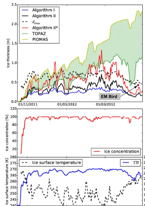
In this section, we analyze the time series of ice thicknesses retrieved from Algorithm I, II, and II* at single grid points in the Laptev Sea and the Beaufort Sea (Point 1: 77.5◦N, 137.5◦E, Point 2: 71.0◦N, 165.0◦W, Point 3: 74.5◦N, 127.0◦E). The time series begin on 15 October 2011. The time series of ice thickness extracted from two different sea ice assimilation systems are included for comparison. In ad-dition, we show time series of SMOS TB together with ice concentration and derived snow/ice surface temperature.

0.0 0.5 1.0 1.5 2.0

Plane layer ice thickness d [m]

0.5 1.0 1.5 2.0

Mean ice thickness H [m]

Sice

=8 gkg

,

=-10

C

Sice

=8 gkg

,

=-5

C

Sice

=1 gkg

,

=-5

C

Figure 10. Relationship between the plane ice layer thicknessdice and the mean inhomogeneous ice layer thicknessHat differentTice andSice. The thin black line is the 1.1 unity line.

The other assimilation system is the Pan-Arctic Ice Ocean Modeling and Assimilation System (PIOMAS) (Zhang and Rothrock, 2003). It is based on a coupled ocean-ice model forced with National Centers for Environmental Prediction Atmospheric Reanalysis data. PIOMAS assimilates satellite-observed sea ice concentration and sea surface temperature data.

At Point 1, which is located in the northern Laptev Sea, Al-gorithm I and II show very similardice, ranging from 0 m to about 0.3 m (Fig. 11) for the first 30 days. The TB increases from about 100 K to about 230 K. In this TB range, dice is the dominant factor of TB variation (Kaleschke et al., 2012). In the next 30 days, TB increases to about 240 K, whereas

diceincreases from about 0.3 m to about 0.4 m in Algorithm I and to more than 0.5 m in Algorithm II. From mid-December to the end of April, TB shows little variability with a mean value of 237.4 K and a standard deviation of 1.9 K. In this period, dice from Algorithm I shows a stable value around 0.35 m with a standard deviation of 3 cm, which results from the constant parameters assumed in Algorithm I. In contrast,

dicefrom Algorithm II shows an average value of 0.48 m with a standard deviation of 11 cm. The strong variability indice is mainly caused byTice. A correlation coefficientRof−0.7 can be found betweenTiceanddice. In the total time period of 200 days,dicefrom Algorithm II is on average 10 cm thicker than that from Algorithm I. The ice thickness corrected with the thickness distribution function (Algorithm II*) is about two times that of Algorithm II.

Simulated ice thicknesses from TOPAZ and PIOMAS show continuous ice growth during the time period, however, with more than 0.5 m span between them (shaded area in the upper panel of Fig. 11). The ice thicknesses retrieved with Algorithm II* correspond well with those from TOPAZ and

Figure 11. Time series of ice thickness derived from Algorithm I,

II, and II*, together withdmaxand simulated ice thicknesses from TOPAZ and PIOMAS (upper panel) and time series of ice concen-tration (middle panel), snow (or ice in the case of bare ice) sur-face temperature and SMOS TB (lower panel) at Point 1 (77.5◦N, 137.5◦E).

PIOMAS in the first three months. However, from March to April TOPAZ and PIOMAS show further growth in the ice thickness, whereas SMOS shows rather constant or decreas-ing trends. The decreasdecreas-ing trend indice corresponds to the decreasingdmaxcaused by the increasingTs.

Point 2 is located in the Beaufort Sea, near Barrow. The first sea ice occurrence happens in mid-November, one month later than at Point 1. A few days after the first occur-rence of sea ice, the ice concentration rapidly reaches nearly 100 % (Fig. 12). In the following 80 days,Tsdecreases from about 270 K to 240 K, anddiceretrieved with Algorithm II* increases from a few centimeters to more than 1.5 m. In this period, the ice thickness growth from SMOS Algorithm II* agrees well with that simulated by TOPAZ and PIOMAS. Just as at point 1, after the three month freeze-up period, the SMOS-retrieveddicereaches its maximum with a decreasing trend in April, which corresponds to the increasingTs.

Figure 12. Time series of ice thicknesses derived from Algorithm I,

II, and II*, together withdmaxand simulated ice thicknesses from TOPAZ and PIOMAS (upper panel) and time series of ice concen-tration (middle panel), snow (or ice in the case of bare ice) sur-face temperature and SMOS TB (lower panel) at Point 2 (71.0◦N, 165.0◦W).

is characterized by large interannual variations, the conse-quence of an enormous freshwater input from the Lena river, and by ice formation and salt rejection processes taking place in polynyas offshore of the fast ice edge. Anticyclonic wind conditions force the riverine water northwards and result in a stronger density stratification in the eastern Laptev sea during winter. Cyclonic atmospheric circulation deflects the freshwater plume of the Lena river eastward towards the East Siberian Sea, thus causing higher salinity in the east-ern Laptev Sea and the area around the West New Siberian (WNS) polynya.

The strong variability of ice thicknesses in SMOS and in the model outputs shows good correlation (Fig. 13). The de-crease and inde-crease of ice thicknesses in SMOS and in the model outputs are very likely caused by the drift of thick ice due to wind forcing and thin ice formation in the polynya areas. From March to April, there is a large discrepancy be-tween the model outputs and the SMOS-derived ice thick-ness. While model outputs show an ice thickness of more

EM Bird

Figure 13. Time series of ice thicknesses derived from Algorithm I,

II, and II*, together withdmaxand simulated ice thicknesses from TOPAZ and PIOMAS (upper panel) and time series of ice concen-tration (middle panel), snow (or ice in the case of bare ice) sur-face temperature and SMOS TB (lower panel) at Point 3 (74.5◦N, 127.0◦E).

than 2 m in April, SMOS-derived ice thickness is less than half a meter.

this assumption may be invalid because the conductivity of saline young ice can be significantly higher than that of older first-year or multi-year ice. This can lead to an underestima-tion of ice thickness.

The survey flight made on 20 April has a length of about 200 km and covers mostly thin ice formed in the WNS polynya and the Anabar–Lena polynya. A period of strong and consistent offshore winds led to the development of an extensive thin ice zone extending several hundred kilometers offshore. Point 3 is located in the middle of the flight track. Therefore, we use the EM-Bird measurements to validate the SMOS-derived ice thickness. During the flights, the EM-Bird recorded a total of 46 386 measurements with a mean value of 43 cm and a standard deviation of 33 cm. This agrees well with the 31 cm ice thickness from SMOS Algorithm II*, con-sidering that the EM-Bird-derived ice thickness is the sum of the thicknesses of the ice layer and the overlying snow. The SMOS ice thickness along the 200 km flight track is quite homogeneous, with a standard deviation of 1 cm. The com-parison shows that in the polynya area, SMOS estimates the ice thickness better than TOPAZ or PIOMAS.

After the time series comparison at single points, we com-pare the daily ice thickness distribution from the three algo-rithms in the Arctic on 1 February 2013. As can be seen in Fig. 14 the mean ice thickness considerably increases from Algorithm I to Algorithm II*. In the central Arctic, which is covered with thick multi-year ice, TB reaches its satura-tion. Therefore, none of the algorithms can deliver reliable ice thickness information in the thick multi-year ice area. If we consider only the pixels where TB has not reached its saturation, ice thickness from Algorithm II* is on average 0.82 m, which is about 40 cm thicker than that from Algo-rithm II and 55 cm thicker than that from AlgoAlgo-rithm I. How-ever, the increase of ice thickness varies from region to re-gion, depending on SSS and weather conditions. For exam-ple, in the Laptev Sea, where the SSS is much lower than that in the central Arctic, the difference between Algorithm II and Algorithm I is as large as half a meter. In contrast, in parts of the Kara Sea and the northern Barents Sea, little change can be observed between Algorithm I and II. The increase of ice thickness in Algorithm II compared to Algorithm I is caused by the deviation of estimatedTiceandSicefrom the constant values assumed in Algorithm I. To investigate the contribu-tion ofTice andSicein the thickness retrieval separately, we carried out two tests with the data from 1 February 2013. In the first test,Siceis assumed to be 8 g kg−1as in Algorithm I and we vary onlyTice. In the second test,Ticeis assumed to be−7◦_{C as in Algorithm I andS}

iceis calculated from SSS. In both tests, we assume a plane ice layer. If we only con-sider the pixels where TB has not reached its saturation, the change of ice thickness caused byTicein Test 1 varies from −10 cm to more than 50 cm, with an average of 11 cm. Larger changes are found where cold air temperatures prevail. The ice thickness change caused bySice from Test 2 is on

aver-Figure 14. SMOS ice thickness derived from retrieval algorithm I,

II, and II* in the Arctic on 1 February 2013.

age 3 cm. However, differences up to 20 cm and 60 cm can be found in the Laptev Sea and in the Baltic Sea.

SMOS-retrieved ice thickness represents both thermody-namic and dythermody-namic evolution of an ice layer, with a spa-tial resolution of about 35 km on a daily basis in the po-lar regions. The variability of SMOS-retrieved ice thickness comes partly from ice drift and ice concentration variation, partly from the changing surface air temperature. We com-pared SMOS ice thickness with PIOMAS and TOPAZ model outputs just to see whether the magnitude of the ice thick-nesses are on the same order. The correlation between SMOS ice thickness and model outputs is low if we remove the sea-sonal cycle. The advantage of the SMOS ice thickness prod-uct is that it can reflect, to some extent, the fine scales of tem-poral and spatial variability of thin ice thickness, which most ocean-sea ice coupled models are not able to simulate. Ice thicknesses derived from a thermodynamic model or from a simple freezing-degree-day ice growth calculation cannot re-flect the variations caused by the ice dynamics which could, however, be captured by SMOS.

The comparison between Algorithm I and II shows that by taking into account the variability of ice temperature and ice salinity, the Arctic-wide ice thickness distribution be-comes more realistic. However, the underestimation of ice thickness caused by the one plane layer assumption is still a shortcoming of Algorithm II. This problem is partly solved in Algorithm II* by implementing a lognormal ice thick-ness distribution function, which is a first approximation of the inhomogeneity of natural ice. The inter-comparison with model outputs shows a considerable advantage of Algorithm II*, which produces ice thickness values close to the model outputs, at least in the freeze-up period. Furthermore, good agreement is found between Algorithm II* and EM-Bird val-idation data in the Laptev Sea. Therefore, Algorithm II* is used to retrieve ice thickness from SMOS data operationally.

7 Ice thickness growth and distribution as seen by SMOS during the freeze-up period

Figure 15. Monthly sea ice thickness derived from Algorithm II*

during the freeze-up period of October 2012 to March 2013 (from upper left to lower right) in the Arctic. Months: October 2012 (up-per left), November 2012 (up(up-per middle), December 2012 (up(up-per right), January 2013 (lower left), February 2013 (lower middle), and March 2013 (lower right).

from October 2012 to March 2013 retrieved with Algorithm II*. From October to November, thin first-year ice extends to most areas of the East Siberian Sea, the Laptev Sea, and the Beaufort Sea. In addition to the area expansion, an increase of ice thickness due to the thermodynamic growth can also be observed. In December, first-year ice reaches a thickness of more than 1 m in the Laptev Sea and the Beaufort Sea. In March 2013, large areas of thin ice with a thickness less than 40 cm are observed in the Beaufort Sea, which is caused by the opening of leads and polynyas in this period.

8 Comparison of SMOS and MODIS ice thickness charts in the Kara Sea

8.1 Sea ice thickness derived from MODIS data For the initial verification of SMOS-retrieved sea ice thick-ness, we use MODIS ice thickness charts for the Kara Sea. The validation extends over an area of 1500 km by 1350 km. The area is suitable for SMOS ice thickness validation be-cause even in the winter time it is frequently covered by thin first-year ice, which SMOS can best detect. To compare SMOS and MODIS ice thicknesses, we reduce the 1 km spa-tial resolution of the MODIS thickness charts to the SMOS ice thickness grid resolution of 12.5 km by spatial averaging. We first compare ice thickness distributions from SMOS and MODIS for two selected days (26 December 2010 and 2 February 2011), on which a sufficient amount of pixels with valid MODIS data is available. After that we collect all pixels with valid MODIS data from 30 days during the two winter seasons 2009–2010 and 2010–2011 and carry out a pixel-to-pixel comparison. The 30 days are selected

man-ually. MODIS ice charts with strong cloud limitation are ex-cluded. We use SMOS Algorithm II for the comparison with ice thicknesses derived from MODIS thermal measurements because both represent the modal (level) ice thickness of un-deformed ice.

8.2 Daily comparison

Figure 16 shows the modal MODIS ice thickness in a 12.5 km grid resolution, the SMOS ice thicknesses re-trieved from Algorithm I and II, and the histogram of the three ice thickness data sets in the Kara Sea on 26 Decem-ber 2010. Ice concentration from the same day (Fig. 17) shows near 100 % ice coverage in the ice-covered area except for the marginal ice zone. Here we use the ice concentration maps derived from SSM/I with the ARTIST Sea Ice (ASI) algorithm. Both SMOS and MODIS show similar patterns of thin and thick ice distributions, whereas SMOS ice thickness from Algorithm I is considerably lower than the other two in the thicker ice range. Surface air temperatureTaover the ice covered area varies from−30 to−20◦C (Fig. 17), pro-viding favorable conditions for both SMOS and MODIS ice thickness retrievals (Kaleschke et al., 2010; Yu and Rothrock, 1996).

The insulation effect of snow is considered in the SMOS Algorithm II and in the MODIS ice thickness retrieval, but not in the SMOS Algorithm I. In Algorithm IITs anddice are retrieved simultaneously with Ta as a boundary condi-tion. The SMOS-derivedTs is in good agreement with that from MODIS (Hall et al., 2004) (Fig. 17). The mean Ts from MODIS and SMOS are both 247 K, and the root mean square deviation (RMSD) is 4 K. Discrepancies can be seen in the marginal ice zone and in the Ob estuary, where the low salinities are not well represented by the ocean model. In the marginal ice zone with lower ice concentrations, SMOS strongly underestimates ice thickness, which leads to too-warmTs. In SMOS Algorithm IITs is used to calculate the bulk ice temperature, which is a variable parameter in the radiation model to calculate the emissivity of an ice layer.

0.0 0.2 0.4 0.6 0.8 1.0 m

30˚ 60˚

90˚

70˚

75˚

20101226 Sea ice thickness

MODIS 0.0 0.2 0.4 0.6 0.8 1.0

[m]

30˚ 60˚

90˚

70˚

75˚

20101226 Sea ice thickness

KlimaCampus SMOS sea ice algorithm I

0.0 0.2 0.4 0.6 0.8 1.0 [m]

30˚ 60˚

90˚

70˚

75˚

20101226 Sea ice thickness

KlimaCampus SMOS sea ice algorithm II

0.0 0.2 0.4 0.6 0.8 1.0

Ice thickness [m] 0.0

0.5 1.0 1.5 2.0 2.5 3.0 3.5 4.0 4.5

Nor

med

occurrence

frequency

SMOS Algorithm I SMOS Algorithm II MODIS in 12.5km resolution MODIS in 1km resolution

Fig. 16.

The modal MODIS ice thickness in 12.5

km

grid resolution (upper left), SMOS ice thicknesses

retrieved from Algorithm I (upper right) and II (lower left), and the histogram of the three ice thickness

data (lower right) in the Kara Sea on 26 December 2010.

55

Figure 16. The modal MODIS ice thickness with 12.5 km grid resolution (upper left), SMOS ice thicknesses retrieved from Algorithm I

(upper right) and II (lower left), and the histogram of the three ice thickness data (lower right) in the Kara Sea on 26 December 2010.

thickness decreases with increasing Tice under cold condi-tions (Maaß, 2013a).

Similar results can be derived from another comparison on 2 February 2011 (see Figs. 18 and 19). On this day, large ar-eas of thin ice can be observed from SMOS and MODIS near the Kara Strait and in the estuaries. In both regions polynyas appear frequently due to the strong wind forcing. Under cold air temperatures, the polynyas are soon covered by thin ice. Both SMOS and MODIS show ice thicknesses in the range of 20–40 cm in the polynyas with similar distribution patterns. Ice concentration is normally higher than 90 % except for the marginal ice zone. As on 26 December 2010, surface air tem-perature over the Kara Sea is as low as−30◦C. In total 4016 pixels have valid MODIS data. The mean ice thickness of

SMOS Algorithm I, SMOS Algorithm II, and MODIS for the pixels are 33 cm, 50 cm, and 47 cm, respectively. The correla-tion coefficient and RMSD between the SMOS Algorithm II and MODIS are 0.61 and 21 cm, whereas between SMOS Al-gorithm I and MODIS they are 0.59 and 26 cm, respectively. The mean surface temperatures from MODIS and SMOS are 246 K and 245 K, with a RMSD of 4 K.

8.3 Comparison with 30 days data from the two winter seasons

0 20 40 60 80 100 [%]

30˚ 60˚

90˚

70˚

75˚

20101226 Sea ice concentration

SSMI/ASI algorithm -40 -30 -20 -10 0 10

[o_C]

30˚ 60˚

90˚

70˚

75˚

20101226 Temperature

JRA25 Reanalysis

240 250 260 270 K

30˚ 60˚

90˚

70˚

75˚

20101226 MODIS

Ice surface temperature 240 250 260 270

[K]

30˚ 60˚

90˚

70˚

75˚

20101226 SMOS

Ice surface temperature

Fig. 17.

SSM/I ice concentration (upper left), JRA-25 surface air temperature (upper right), MODIS- and

SMOS-based snow/ice surface temperature (lower left and lower right) in the Kara Sea on 26 December

2010.

56

Figure 17. SSM/I ice concentration (upper left), JRA-25 surface air temperature (upper right), MODIS- and SMOS-based snow/ice surface

temperature (lower left and lower right) in the Kara Sea on 26 December 2010.

with usable MODIS data. Therefore, we selected out 30 days during which the data are not badly affected by cloud cover-age. Altogether, 81 350 pixels are available at 12.5 km reso-lution. The histogram of the ice thicknesses (Fig. 20) shows better agreement between SMOS Algorithm II and MODIS than between SMOS Algorithm I and MODIS for these pix-els. The mean ice thicknesses derived from SMOS Algorithm II and MODIS are of similar magnitude – 44 cm and 42 cm, respectively, whereas SMOS Algorithm I shows 31 cm on average. If we restrict the comparison to the pixels with MODIS ice thicknesses less than 50 cm, the mean ice thick-ness from SMOS Algorithm II is about 13 cm higher than the MODIS mean value (see Table 2). The spatial correlation

co-efficient between SMOS and MODIS is on average about 0.6 for the selected days.

9 Conclusions

0.0 0.2 0.4 0.6 0.8 1.0 m

30˚ 60˚

90˚

70˚

75˚

20110202 Sea ice thickness

MODIS 0.0 0.2 0.4 0.6 0.8 1.0

[m]

30˚ 60˚

90˚

70˚

75˚

20110202 Sea ice thickness

KlimaCampus SMOS sea ice algorithm I

0.0 0.2 0.4 0.6 0.8 1.0 [m]

30˚ 60˚

90˚

70˚

75˚

20110202 Sea ice thickness

KlimaCampus SMOS sea ice algorithm II

0.0 0.2 0.4 0.6 0.8 1.0

Ice thickness [m] 0

1 2 3 4 5

Nor

med

occurrence

frequency

SMOS Algorithm I SMOS Algorithm II MODIS in 12.5km resolution MODIS in 1km resolution

Fig. 18.

The modal MODIS ice thickness in 12.5

km

grid resolution (upper left), SMOS ice thicknesses

retrieved from Algorithm I (upper right) and II (lower left), and the histogram of the three ice thickness

data (lower right) in the Kara Sea on 2 February 2011.

57

Figure 18. The modal MODIS ice thickness in 12.5 km grid resolution (upper left), SMOS ice thicknesses retrieved from Algorithm I (upper

right) and II (lower left), and the histogram of the three ice thickness data (lower right) in the Kara Sea on 2 February 2011.

(Algorithm I) (Kaleschke et al., 2012), in which a constant

Tice(−7◦C) andSice(8 g kg−1) are assumed. The new algo-rithm allows the retrieval of considerably higher thicknesses for cold conditions and less saline ice. The maximal retriev-able ice thicknessdmaxcan be estimated based on theTiceand Siceat each pixel. In contrast, we estimatedmaxto about 0.5 m as a constant upper limit for the ice thickness retrieval with Algorithm I. In Algorithm II, dmax varies from a few cen-timeters to about 1 m, depending on theTice andSice. A TB saturation factor is defined as the ratio ofdicetodmaxfor each pixel. A saturation ratio close to 100 % indicates that the re-trieved ice thickness must be considered as a minimum ice thickness and that the upper bounds of uncertainty cannot be constrained by the SMOS measurement alone.

0 20 40 60 80 100 [%]

30˚ 60˚

90˚

70˚

75˚

20110202 Sea ice concentration

SSMI/ASI algorithm -40 -30 -20 -10 0 10

[o_C]

30˚ 60˚

90˚

70˚

75˚

20110202 Temperature

JRA25 Reanalysis

240 250 260 270 K

30˚ 60˚

90˚

70˚

75˚

20110202 MODIS

Ice surface temperature 240 250 260 270

[K]

30˚ 60˚

90˚

70˚

75˚

20110202 SMOS

Ice surface temperature

Fig. 19.

SSM/I ice concentration (upper left), JRA-25 surface air temperature (upper right), MODIS- and

SMOS-based snow/ice surface temperature (lower left and lower right) in the Kara Sea on 2 February

2011.

58

Figure 19. SSM/I ice concentration (upper left), JRA-25 surface air temperature (upper right), MODIS- and SMOS-based snow/ice surface

temperature (lower left and lower right) in the Kara Sea on 2 February 2011.

The ice thickness from Algorithm II* agrees well with those from the assimilation systems TOPAZ and PIOMAS in the three months after the first occurrence of sea ice. How-ever, from March to April, TOPAZ and PIOMAS have much higher ice thicknesses compared to the SMOS retrieval. The discrepancy coincides with the onset of surface warming. We observe a strong impact ofTiceon the ice thickness retrieval when TB approaches saturation. The emissivity model used here does not correctly account for vertical gradients of tem-perature and salinity. The invalid assumption of a vertically homogeneous ice layer introduces significant uncertainties because the relative brine volume and thus the permittivity depends on ice temperature and salinity (Maaß, 2013a). More work has to be done to develop and test parameterizations

that could account for the effects of a vertically structured sea ice cover to further improve the emissivity model. How-ever, a validation with EM-Bird measurements in the polynya areas of the Laptev Sea in April 2012 shows very good agree-ment between EM-Bird and SMOS ice thicknesses, whereas TOPAZ and PIOMAS overestimate the ice thickness by 0.5– 2 m.

0.0 0.2 0.4 0.6 0.8 1.0 Ice thickness [m]

0.0 0.5 1.0 1.5 2.0 2.5 3.0 3.5 4.0

Nor

med

occurrence

frequency

SMOS Algorithm I SMOS Algorithm II MODIS in 12.5 km resolution MODIS in 1 km resolution

Figure 20. Histogram of SMOS (Algorithm I and II) and MODIS

(in 12.5 km and 1 km grid resolution) ice thicknesses from all pixels of the selected 30 days between 2009 and 2011.

MODIS retrievals on the SMOS grid by taking the modal mean. The different integration times (SMOS: daily aver-ages vs. MODIS: single overpasses) introduce additional un-certainties. Nevertheless, the ice thicknesses retrieved from SMOS and MODIS are very similar, with a considerably bet-ter agreement between SMOS Algorithm II and MODIS. The correlation coefficientRbetween SMOS and MODIS data is about 0.6 for both Algorithm I and II.

The retrieval uncertainty is dominated by inaccurate as-sumptions and boundary conditions obtained from auxiliary data, whereas the radiometric accuracy is well constrained and sufficient, except for RFI-affected areas. Factors that af-fect the ice thickness retrieval include the ice concentration, ice salinity, ice temperature, snow thickness as well as the statistical thickness distribution function. Sea ice concen-tration data available from passive microwave sensors like the Special Sensor Microwave Imager/Sounder (SSMIS) and the Advanced Microwave Scanning Radiometer 2 (AMSR2) have an inherent uncertainty of about 2.5–5 % over high-concentration ice in winter and have strong limitations in new-ice areas (Andersen et al., 2007; Ezraty, 2002). Thus, we do not correct for varying ice concentration because this would considerably increase the noise and raise as of yet un-resolved problems in regions where new ice is not detected with traditional methods but only with SMOS. The variabil-ity of the sea surface salinvariabil-ity contributes only a little to the overall uncertainty except for low-salinity areas. By ignor-ing the growth-rate dependent salt inclusion in Ryvlin’s pa-rameterization, we introduce additional errors that can not be quantified without the use of more advanced sea ice thermodynamic models (Notz and Worster, 2009; Vancop-penolle et al., 2006). The radiation model used in this study is adapted from Menashi et al. (1993), which is a simple

one-layer model without a snow one-layer. Although we consider the insulation effect of snow, the radiative contribution of the snow layer to the overall brightness temperature is ignored. This effect is investigated in Maaß et al. (2013b) with another radiation model based on Burke et al. (1979). The quantifi-cation of the effect and uncertainty caused by snow layers is considered as future work.

MODIS-based thin ice thickness retrieval is heavily re-stricted by clouds and distinguishing clear sky from clouds is nowhere more difficult than in winter nighttime conditions (Frey et al., 2008). Manual methods are typically needed to improve detection of thin clouds and ice fog (Maekynen et al., 2013). Distinct advantages of the SMOS sea ice thick-ness retrieval are the daily coverage, independent of clouds, and the large sensitivity for thin ice. Thus, our SMOS prod-uct is complementary to the sea ice thickness derived from CryoSat-2 and feasible for operational usage. However, the thickness retrieval is strictly limited to cold periods and not applicable during late spring and summer. Daily SMOS ice thickness charts from 15 October to 15 April from 2010 on are available via http://icdc.zmaw.de.

Acknowledgements. This work was funded through ESA’s Support

to Science Element Program under contract 4000101476. The authors would like to thank the members of the ESA SMOSIce project for helpful discussions. EM-Bird thickness measurements were conducted by the Alfred Wegener Institute for Polar and Ma-rine Research (Thomas Krumpen and Valeria Selyuzhenok) within the Transdrift XX campaign in the framework of Russian-German research cooperation. JRA-25 reanalysis data are provided by the Japanese Meteorological Agency (JMA), the sea ice concentration data are provided by ICDC University of Hamburg, TOPAZ data are provided by Laurant Bertino from the Nansen Environmental and Remote Sensing Center in Norway, and PIOMAS data are provided by Jinlun Zhang from the University of Washington. The authors would like to thank two anonymous reviewers and the editor for their constructive comments.

Edited by: J. Stroeve

References

Andersen, S., Tonboe, R., Kaleschke, L., Heygster, G., and Peder-sen, L.: Intercomparison of passive microwave sea ice concen-tration retrievals over the high-concenconcen-tration Arctic sea ice, J. Geophys. Res., 112, C08004, doi:10.1029/2006JC003543, 2007. Antonov, J., Seidov, D., Boyer, T., Locarnini, R., Mishonov, A., Garcia, H., Baranova, O., Zweng, M., and Johnson, D.: World Ocean Atlas 2009, Vol. 2, Salinity, edited by: Levitus, S., 184 pp., US Gov. Print. Off., Washington, DC, 2010.

Bertino, L. and Lisæter, K. A.: The TOPAZ monitoring and predic-tion system for the Atlantic and Arctic Oceans, Journal of Oper-ational Oceanography, 1, 15–19, 2008.

Brath, M., Scharffenberg, M. G., Serra, N., and Stammer, D.: Altimeter-based estimates of eddy variability and eddy transports in the subpolar North Atlantic, Mar. Geod., 33, 472–503, 2010. Burke, W., Schmugge, T., and Paris, J.: Comparison of 2.8-and

21-cm microwave radiometer observations over soils with emission model calculations, J. Geophys. Res., 84, 287–294, 1979. Camps, A., Vall-llossera, N., Duffo, N., Torres, F., and Corbella, I.:

Performance of sea surface salinity and soil moisture retri