Level 1 algorithms for TANSO on GOSAT: processing and on-orbit calibrations

(1)

Atmos. Meas. Tech., 5, 2447–2467, 2012 www.atmos-meas-tech.net/5/2447/2012/ doi:10.5194/amt-5-2447-2012

Atmospheric

Measurement

Techniques

Level 1 algorithms for TANSO on GOSAT:

processing and on-orbit calibrations

A. Kuze1, H. Suto1, K. Shiomi1, T. Urabe1, M. Nakajima1, J. Yoshida2, T. Kawashima2, Y. Yamamoto3, F. Kataoka4, and H. Buijs5

1_{Japan Aerospace Exploration Agency, Tsukuba-city, Ibaraki, Japan} 2_{NEC Toshiba Space Systems, Ltd., Fuchu, Tokyo, Japan}

3_{NEC Informatec Systems, Ltd., Kawasaki-City, Kanagawa, Japan}

4_{Remote Sensing Technology Center of Japan, Tsukuba-city, Ibaraki, Japan} 5_{ABB, Inc., Quebec-city, Quebec, Canada}

Correspondence to: A. Kuze ([email protected])

Received: 5 February 2012 – Published in Atmos. Meas. Tech. Discuss.: 24 April 2012 Revised: 18 September 2012 – Accepted: 19 September 2012 – Published: 19 October 2012

Abstract. The Thermal And Near infrared Sensor for car-bon Observation Fourier-Transform Spectrometer (TANSO-FTS) onboard the Greenhouse gases Observing SATellite (GOSAT) (nicknamed “Ibuki”) has been providing global space-borne observations of carbon dioxide (CO2) and

methane (CH4) since 2009. In this paper, we first describe

the version V150.151 operational Level 1 algorithms that produce radiance spectra from the acquired interferograms. Second, we will describe the on-orbit characteristics and cal-ibration of TANSO-FTS. Overall function and performance such as signal to noise ratio and spectral resolution are within design objectives. Correction methods of small on-orbit degradations and anomalies, which have been found since launch, are described. Lastly, calibration of TANSO Cloud and Aerosol Imager (TANSO-CAI) are summarized.

1 Introduction

1.1 Overview

The Greenhouse gases Observing SATellite (GOSAT) was successfully launched into a sun-synchronous orbit on 23 January 2009 to monitor global distributions of carbon dioxide (CO2)and methane (CH4). GOSAT carries two

in-struments, namely, the Thermal And Near infrared Sen-sor for carbon Observation Fourier-Transform Spectrometer FTS) and the Cloud and Aerosol Imager

(TANSO-CAI). TANSO-FTS measures reflected solar radiance in the oxygen (O2)A band region at 0.76 µm (Band 1) and in the

weak and strong CO2bands at 1.6 µm (Band 2) and 2.0 µm

(Band 3) respectively, and also CH4bands at 1.67 µm (Band

2) all with two orthogonal linear polarizations, designated “P” and “S”. TANSO-FTS also measures spectral radiance in the thermal IR (Band 4). TANSO-CAI has four spec-tral bands, namely, 0.380 µm (Band 1), 0.674 µm (Band 2), 0.870 µm (Band 3), and 1.60 µm (Band 4) to determine clear soundings of the TANSO-FTS measurements and to provide cloud and aerosol optical properties.

GOSAT is a joint project of the Japan Aerospace Explo-ration Agency (JAXA), Ministry of the Environment (MOE) and the National Institute for Environmental Studies (NIES). JAXA is responsible for producing the Level 1A (raw inter-ferogram) and the Level 1B (radiance spectra) products of TANSO-FTS and the Level 1A (raw digital image) product of TANSO-CAI. NIES provides the Level 2 (CO2and CH4

concentrations from Level 1B spectra), the Level 3 (global distribution of CO2 and CH4 concentrations by

interpolat-ing the Level 2 products), and the Level 4 (net CO2sources

(2)

2448 A. Kuze et al.: Level 1 algorithms for TANSO on GOSAT

Page 1/20

Fig.1. The schematics of the TANSO-FTS and CAI optics modules.

Copernicus Publications

Bahnhofsallee 1e

Contact

[email protected]

Legal Body Copernicus Gesellschaft mbH 37081 Göttingen

Germany

Martin Rasmussen (Managing Director) Nadine Deisel (Head of Production/Promotion)

http://publications.copernicus.org Phone +49-551-900339-50 Fax +49-551-900339-70

Based in Göttingen Registered in HRB 131 298 County Court Göttingen Tax Office FA Göttingen USt-IdNr. DE216566440

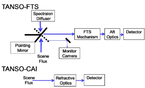
Fig. 1. The schematics of the TANSO-FTS and CAI optics modules.

and responsible institute are summarized in Table 1. All sig-nals (Level 0) transmitted from the GOSAT satellite are re-ceived at Kongsberg Satellite Services AS (KSAT), Norway and Earth Observation Center (EOC), Japan and transmit-ted to Tsukuba Space Center (TKSC), Japan. Thereafter, the TANSO-FTS Levels 1A and 1B data and the TANSO-CAI Level 1A data are produced at TKSC. Usually the Level 1 data is transferred to NIES and other users such as the Na-tional Aeronautics and Space Administration (NASA) in the United States and the European Space Agency (ESA) within 5 h after the initial observation on orbit. The Level 1B data together with all the necessary calibration and correction data and the higher data products produced in NIES are available at the NIES GOSAT User Interface Gateway (GUIG). Data of a monitor camera (CAM) (see Fig. 1) are not processed as a Level 1 product because it was originally installed to check pointing mirror alignment onboard after launch, espe-cially the difference between the actual viewing position and the calculated value from the resolver of the pointing mirror mechanism. We describe here the data processing algorithms of the TANSO Levels 1A and 1B. The details of the Level 2 algorithms are described in Yoshida et al. (2011) for TANSO-FTS short wave infrared (SWIR) bands, Saitoh et al. (2009) for the thermal infrared (TIR) band, and Ishida et al. (2009, 2011) for TANSO-CAI.

1.2 TANSO Instruments

The schematics of the TANSO-FTS and CAI optics mod-ules are illustrated in Fig. 1. TANSO-FTS has many func-tions and operational modes. The two-axis pointing mech-anism has pointing and image motion compensation func-tions, allowing precise viewing of the Earth and the calibra-tion sources. In nominal observacalibra-tion mode, the pointing mir-ror views predefined grid points of the Earth close to nadir as illustrate in Fig. 2. In the sun-glint observation and spe-cial target modes, the pointing mirror views the specular reflection points over the ocean and requested observation points, respectively. The FTS scan mechanism sweeps the optical path difference (OPD) of the interferometer. The

per-Table 1. TANSO-FTS data product format. Data level, data product, data format, and responsible institution.

Data Data Data Responsible

level product format institute

1A Raw interferograms HDF JAXA

1B Spectral radiance HDF JAXA

2 XCO2andXCH4

soundings

HDF NIES

3 Global distribution

ofXCO2 andXCH4

HDF NIES

4 CO2sources/sinks NetCDF NIES

formance of these two mechanisms on orbit has been care-fully characterized and is described in Sects. 2.3.3 and 3.4. TANSO-CAI is a much simpler instrument. It has no me-chanical moving parts and no onboard calibrator. It views a wide swath of 910 km and acquires a global image in 3 days. The spectral and geometric performance of TANSO-CAI on orbit is assumed to be stable. During the daytime both SWIR and TIR of TANSO-FTS and TANSO-CAI data are acquired. During the nighttime only TANSO-FTS TIR data are ac-quired. Overall the radiometric responses of both TANSO-FTS and CAI are the combination of the optical efficiency, detector response, and the gain of the analog circuits. The on-orbit response changes have been monitored for three years and their characterization is described in this paper. Details related to each instrument design, prelaunch hardware per-formance, and on-orbit operations were described in Kuze et al. (2009).

1.3 GOSAT operation

The function and performance of all systems were veri-fied to meet operating standards during the initial three-month checkout phase after launch (January to mid-April 2009). In the second three-month phase (May to July 2009), the initial calibration was performed. During this period, the first vicarious calibration campaign was per-formed and the responses of TANSO-FTS and CAI were cal-ibrated (Kuze et al., 2011a). The nominal operation phase started in July 2009. More than three years have passed since launch, and the overall functions and performances are within design objectives. All measured radiance spec-tra of the TANSO-FTS SWIR and TIR bands and column-averaged dry air mole fractions (the Level 2 product) of CO2

and CH4 (XCO2 andXCH4, respectively) retrieved from the

SWIR bands are currently available to the public from NIES. In addition to the standard GOSAT Level 2 product provided by NIES, several other working groups have derivedXCO2

andXCH4 from the TANSO Level 1 data using their own

(3)

A. Kuze et al.: Level 1 algorithms for TANSO on GOSAT 2449

Page 2/20

(a) (b)

(c)

Fig.2.Grid observation patterns: (a) 5-pointcross-track scan mode (b) a M shape

grid overwritten on 5-pointcross-trackscan mode, and (c) 3-pointcross-track scan

mode.

Copernicus Publications Bahnhofsallee 1e

Contact

[email protected]

Germany

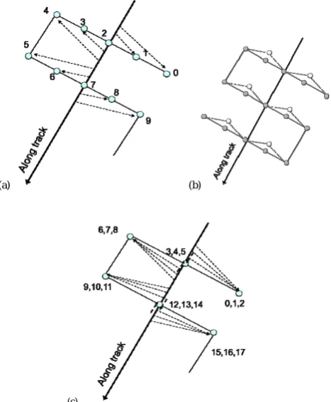
Fig. 2. Grid observation patterns: (a) 5-point cross-track scan mode (b) a M shape grid overwritten on 5-point cross-track scan mode, and (c) 3-point cross-track scan mode.

space for the first time using high-spectral-resolution Fraun-hofer line spectra by Joiner et al. (2011, 2012), Frankenberg et al. (2011a, b), and Guanter et al. (2012).

GOSAT has a 3-day revisit orbit cycle and a 12-day op-eration cycle. Three different opop-erational patterns have been employed to insert target observations into nominal grid ob-servations. These are pattern A, consisting of limited calibra-tion and validacalibra-tion site observacalibra-tions; pattern B, consisting of sun glint over the ocean near the sun’s declination as well as target observations requested by registered researchers re-sponding to research announcements (RA); and pattern C, consisting of sun glint and limited calibration and validation site observations. Each pattern is maintained for three days and the repeated order of the patterns is A, B, C, and B. The detailed operation modifications in chronological order were described in Kuze et al. (2011b).

Several anomalies were found in on-orbit operation of TANSO-FTS and the operation was modified to avoid per-formance degradation (Kuze et al., 2011c). One of the ma-jor anomalies is the zero path difference (ZPD) shift, which degrades the spectral resolution and needs to be corrected. ZPD is the center of the interferogram. The FTS scan arm is servo-controlled using monochromatic laser fringes. This achieves uniform-speed scanning within the OPD range fol-lowed by rapid reversal of the scan-arm motion (turnaround).

The fringe count is also used to trigger the turnaround of the scan mechanism at precisely repeatable scan distance from ZPD. This is done by up and down counting accord-ing to scan direction. Duraccord-ing turnaround, both FTS scan and pointing mirror are activated simultaneously. A combi-nation of microvibrations caused by the pointing motion, a slower speed scan at turnaround and in an electro-magnetic-noise environment, has reduced the reliability of the fringe count which occasionally causes the controller of the FTS-mechanism to miss count the laser fringes at the turnaround position and consequently causes the ZPD position to shift gradually. Now periodically the ZPD position is reset by up-loading a fringe shift command from the ground. The shifted fringe number is recorded in the Level 1B product.

The other major anomaly is a pointing bias of the pointing mirror, which may be due to a bias of the angular resolver (an angular position sensor) or insufficient electrical power to properly drive the along track (AT) motor. Also, within the AT motion range, there are several “dead band” zones, where the AT motion becomes unstable or even occasion-ally settles down in an incorrect position. The 2nd and 4th of the original five cross-track (CT) points shown in Fig. 2a are close to dead band angles and they have large biases: in some cases they can be detected by the resolver and then can be geometrically corrected. Instead of the nominal 5-point grid, an M shape pattern as illustrated in Fig. 2b was introduced between 26 June 2009 and 31 July 2010. This is to avoid the dead band areas and to minimize the pointing anomalies. The exact pointing locations of the M shape can be retrieved in the Level 1B geolocation data. With a simple 3-point cross-track pattern as shown in Fig. 2c dead band zones are also avoided. Therefore, a simpler 3-point cross-track scan mode has been employed more recently. The trend of the bias and the geometric collection method using camera data are to be described later.

Between launch and July 2010, for the 5-point cross-track scan mode, interferograms had been acquired every 4.45 s (4 s for interferogram acquisition and 0.45 s for turnaround). This resulted in 150 km spacing between grid observations and a total of 56 000 soundings globally every three days. Since August 2010, the grid observation pattern has changed from the 5-point track scan mode to the 3-point cross-track scan mode with 260 km spacing. Implementation of a longer turnaround time of 0.6 s probably decreased the ZPD shift rate as well. The sun glint observation uses the image motion compensation (IMC) to minimize the input intensity fluctuation and to reduce the cloud contamination.

(4)

characterization of on-orbit, onboard and vicarious calibra-tions are presented. Lastly, TANSO-CAI characterization and calibration are described in Sect. 4.

2 TANSO-FTS Level 1 algorithm

In this section, the version V150.151 TANSO-FTS Level 1 algorithm is described. The algorithm has been updated sev-eral times since launch. The versions in chronological order were described in Kuze et al. (2011b).

All the unprocessed numerical form interferograms are saved as Level 1A data. The payload correction data from the satellite bus and telemetry data of TANSO-FTS are added in both Levels 1A and 1B products together with the mea-sured data. These data include the time stamp, the satellite and sun position, the geolocation, the AT and CT angles of the pointing mirror, the detector temperature, the blackbody temperature, and gain level, all of which are necessary for the data processing and analysis. The time stamp in the data shows the start of the interferogram acquisition. The satellite position is interpolated by using the payload correction data, which is transmitted from the satellite every second. The AT, CT, solar angles, and the geometry information are acquired at the start of the interferogram acquisition as well.

2.1 Procedures

Interferograms of each band (two linear polarizations of bands 1, 2, and 3 and scalar band 4) are processed indepen-dently. TANSO-FTS bands 1, 2 and 3 (SWIR) are processed as follows:

Step S1: Saturation detection

Step S2: Correction of spikes caused by cosmic rays hitting the detector

Step S3: Scan speed instability correction (applied for the Band 1 medium gain only)

Step S4: Intensity variation correction (bands 2 and 3 only) Step S5: OPD sampling interval non-uniformity correction Step S6: Direct current (DC) subtraction and ZPD detection Step S7: Inverse fast Fourier transform (IFFT)

Step S8: Phase correction

Step S9: Analog circuit nonlinearity correction. TANSO-FTS Band 4 (TIR) is processed as follows: Step T1: Saturation detection

Step T2: Nonlinearity correction of the Band 4 photo conduc-tive (PC) – mercury cadmium telluride (MCT) detector

Step T3: Correction of spikes caused by cosmic rays hitting the detector

Step T4: OPD sampling interval non-uniformity correction Step T5: ZPD detection

Step T6: IFFT

Step T7: Complex radiometric calibration and deep space (DS) view obscuration correction

Polarization correction of the pointing mirror.

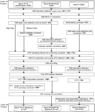
A detailed flow diagram is shown in Fig. 3 and each pro-cess is explained in the following subsections.

2.2 Introductory remarks

On the TANSO-FTS, interferograms are measured on both sides of the ZPD position providing “double-sided” interfer-ograms. Furthermore the three SWIR bands are quite narrow compared to their center wavelength in order to minimize un-necessary photon noise. At the same time the interferograms are sampled at high OPD density compared with the band-width of each band. There is no onboard data compression. The result is that the out of band zero parts of the result-ing spectra as well as the imaginary component of the spec-trum provide a sensitive check on saturation, nonlinearity, and OPD sampling uniformity.

2.3 Corrections

2.3.1 Saturation, low frequency fluctuation, and spike detection, and correction (Steps S1, S2, T1, and T3)

(5)

Fig. 3.

Fig. 3. The TANSO-FTS Level 1 data processing flow. Steps S1–S9 and T1–T5 are indicated in bold letters.

spikes are removed and filled with an estimated DC signal, which is the average of the interferogram levels acquired be-fore and after the spike.

2.3.2 Digitization and its nonlinearity

Nonlinearity of the raw interferogram readout requires cor-rection. There are three blocks in the signal electronics: namely the detector, analog circuit, and ADC. The Si detec-tors of Band 1 and InGaAs detecdetec-tors of bands 2 and 3 are adequately linear. The Band 4 PC-MCT detector has nonlin-earity, and its correction method is described in Sect. 2.3.7.

The analog circuit consists of the current-to-voltage con-verter (transimpedance amplifier), gain amplifier, and elec-tric filters: their characteristics and correction are described in Sect. 2.3.6.

(6)

Page 5/20

Fig.4.ADC integral non-uniformity correction value retrieved from the measured

data using the engineering model.

Bahnhofsallee 1e

Contact

[email protected]

Germany

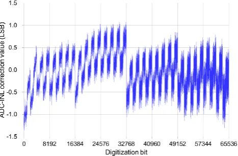
Based in Göttingen Registered in HRB 131 298 County Court Göttingen Tax Office FA Göttingen USt-IdNr. DE216566440 Fig. 4. ADC integral non-uniformity correction value retrieved from the measured data using the engineering model.

their differential nonlinearity (DNL) and integral nonlinear-ity (INL). A DNL larger than 1 bit becomes a missing code. By measuring DNL bit by bit, the INL of the entire dynamic range can be characterized. Figure 4 shows the INL correc-tion value retrieved from measured data using the TANSO-FTS engineering model. ADC nonlinearity produces spectral artifacts, which vary with the intensity level of the input flux. The 16-bit ADCs used in TANSO-FTS have the largest non-linearity at the center of the dynamic range. The Band 1 sig-nals are alternating current (AC) coupled and the center bit is frequently used as OPD increases. Although INL of the entire dynamic range has been characterized, it has proven very difficult to correct the ADC nonlinearity particularly for low level AC sampled interferograms. In version V130.130 (the previous version of Level 1B processing) correction of the ADC nonlinearity was attempted. However in the case of low input signal, the resulting Level 1B products suffered from large artifacts. Therefore, the version V150.151 does not correct the ADC nonlinearity. As a result, in the case of very low signal flux, the Level 1B data of Band 1 may have a possible small bias.

2.3.3 Correction of scan speed instability (Step S3)

The phase delay mismatch between the metrology laser elec-tronics and science channel degrades the robustness to scan speed instability and creates artifacts in the spectra. Only the medium gain of Band 1, which is used over high reflectance regions such as the Sahara, Arabian and Australian deserts and solar calibration, has a significant delay mismatch: group delays of high and medium gains are different and the delay matching is applied only to high gain. When speed instabil-ity is large, the Band 1 interferogram with the medium gain is not uniformly sampled. In the worst case, the sampling interval changes by about±0.6 % and the spectral radiance changes by±1.5 %. The speed instability is caused by a com-bination of two sinusoidal microvibration sources, namely, a

244 Hz from the satellite attitude control’s Earth sensor and the 325.5 Hz resonant frequency of the FTS mechanism. Ex-cept for these two oscillations, the on-orbit mechanical envi-ronment is very quiet. Since the nominal scan speed is very constant, these two additional modulations to the interfero-gram have quite pure sinusoidal variations and can be cor-rected by retrieving their amplitudes and phases for each in-terferogram acquired with medium gain. As each interfer-ogram is processed, these four parameters are estimated to minimize the out-of-band artifact spectra. The interferogram is then interpolated at the expected sampling positions but at the cost of additional computation resources in the ground data processing (Simon, 2008; Suto and Kuze, 2010). After applying the correction introduced in Version 110.110, the standard deviation of the Band 1 medium gain data has been significantly reduced to the noise level (Suto et al., 2011a). 2.3.4 Correction of the intensity variation component

(Step S4)

The acquisition of both modulated and non-modulated por-tions of the DC coupled interferogram of bands 2 and 3 is performed in order to check the data quality. The metrology wavelength of TANSO-FTS is 1.31 µm. Even sampling the OPD at half the wavelength by means of up-and-down zero-crossings of laser fringes, the wavelength of Band 1 is still shorter than twice the sampling interval and hence Band 1 frequencies are aliased to low frequencies. Both optical and electrical filters are employed to minimize aliased signal and noise mixing. This also necessitates AC coupling of the sig-nal to the ADC and hence preventing the data quality deter-mination as is done for bands 2 and 3. Band 4 is also AC sampled to reduce the non-modulated background radiation. By checking the DC coupled interferogram, changes in the scene radiant intensity such as erratic intensity changes due to the pointing anomaly can be detected. DC coupled inter-ferograms may also show low frequency variations which are indicative of pointing jitter and optical vignetting. These fre-quencies are typically lower than 500 Hz and much lower than the scene signal modulation of the interferometer which is of the order of 10 KHz. They have independent amplitude and phase and can be extracted from the interferogram. We remove the low frequency component by dividing an inter-ferogram created from the low frequency components. This method is similar to the method applied to the FTS units of the Total Carbon Column Observing Network (TCCON) (Keppel-Aleks et al., 2007).

(7)

Page 6/20

-2 -1 0 1 2 -15 -10 -5 0 5 10 OPD (cm) Diff fr om exp ec te

d to mea

s u red OPD (nm) Backward scan Forward scan D ev ait ion f rom t h e ideal s am pling point (nm )

Optical path difference (cm)

Fig.5.Sampling interval non-uniformity as a function of OPD of the forward and

backward scans. Copernicus Publications Bahnhofsallee 1e Contact [email protected] Legal Body Copernicus Gesellschaft mbH 37081 Göttingen

Germany

Fig. 5. Sampling interval non-uniformity as a function of OPD of the forward and backward scans.

are corrected. The field of view of TANSO-FTS is too large to permit realization of the full resolution for Band 1. The in-terferograms of Band 1 undergo strong self-apodization and as a result Band 1 has a different resolution compared with bands 2, 3, and 4.

The second contribution is scene flux fluctuation due to the constant satellite sinusoidal vibration motion. The typical frequency is about 10 Hz and the possible source is the satel-lite’s reaction wheel. The last contribution is the pointing mirror fluctuation, which occurs irregularly. About 20 % of the total interferograms are affected by the fluctuation caused by the pointing mirror and have intensity modulation. We can detect these two fluctuations by checking the Band 2 inter-ferograms. If the scene is spatially uniform, we cannot detect the pointing mirror fluctuations. At the same time, the spec-tra of the spatially uniform targets are not affected by these fluctuations.

2.3.5 Correction of OPD sampling interval non-uniformity (Steps S5 and T4)

The ideal interferogram of the scene flux would be acquired with equal sampling intervals of the laser fringes within the entire OPD range. The actual on-orbit interval decreases by only 25 nm from ZPD to maximum OPD. The change is not linear with OPD, and the forward and backward scans of the FTS mechanism are slightly different as shown in Fig. 5. The error caused by this non-uniformity is close to the noise level in the forward direction data but slightly larger in the back-ward scan data. The root cause is not well-known, but it is probably caused by the laser optical misalignment, asymme-try of the FTS scan-mechanism structure, and its electronic control imperfection. The deviation on orbit can be estimated by analyzing the onboard ILSF calibration laser data. As the deviation is reproducible on orbit, this non-uniformity is corrected by resampling the interferogram.

2.3.6 Correction of Band 1 analog circuit nonlinearity (Step S9)

The high gain of Band 1 uses a Chebyshev filter with much sharper gain peak and cutoff than the other bands to avoid aliasing of noise. Unfortunately, its gain is sensitive to the capacitance in the circuit, which varies with input voltage, temperature, and time. Apart from the high gain Band 1, all bands use Butterworth filters, which have flat responses. Changes in their feedback capacitance result only in small shifts in their cutoff. The nonlinearity induced by the input-voltage change can be corrected using a 3rd order polyno-mial (Suto et al., 2011b). These coefficients are determined such that the out-of-band artifact spectra are minimized. The nonlinearity is a function of both the input voltage and the ZPD level. Thus, the nonlinearity is corrected after the phase correction as indicated in Fig. 3. We have prepared the 3rd-order-coefficient tables as a function of the ZPD voltage. Temperature dependency might cause seasonal and orbit phase changes and the time dependency might cause long-term changes. Band 1P has shown an especially larger change and these effects need further investigation. We re-placed the capacitor of the engineering model with a temper-ature compensated one in the laboratory on the ground and then the artifact spectra were removed. These test results also indicate that our correction algorithm works well.

2.3.7 Correction of TIR detector nonlinearity (Step T2)

We use a photo-conductive PC-MCT detector, which has nonlinearity for strong signal input for Band 4. The nonlin-earity can be corrected using a 2nd order polynomial. As-suming that nonlinearity characteristics do not change with time after launch, the coefficients can be determined from the well-characterized large photon input data under stable conditions in a vacuum chamber prior to launch. There are two ways to find the correction parameters. When the detec-tor and its analogue electronics have nonlinearity, the largest signal at ZPD is distorted and artifact low frequency spectra are created. The correction coefficients are tuned such that in-terferograms filtered to have only low frequency components are flat near ZPD. The other method is to select the correction coefficients to fit the artifact shape at the edges of the band, i.e. 300–600 cm−1and 2200–3500 cm−1. The latter method is applied as it has greater sensitivity to determine the coeffi-cients. They are fine-tuned such that corrected signals of the out-of-band region are flat. The nonlinearity corrected data

VNLcorrected is calculated by Eqs. (1) and (2) described

be-low with measured raw AC components of the interferogram in voltageVAC and DC voltageVDC.VDCis the average of

DC samples, which are monitored at 38 samples per inter-ferogram. We subtract offsetVDCoffset, which has a gradual

(8)

data and modeled as a function of time since launch.

VPamp= −((VDC−VDCoffset)/gDC)−VAC/gAC. (1)

The gain factorsgDCandgACare 0.681 and 110.103,

respec-tively.

VNLcorrected=VPamp+anlcVPamp2 . (2)

anlcis the nonlinearity correction coefficient of 0.6056.

2.4 Inverse fast Fourier transform

2.4.1 ZPD detection and inverse fast Fourier transform (Steps S6, S7, T5, and T6)

The ZPD position is determined by searching the center burst (peak) of the interferogram. The interferogram is then con-verted to the spectra with a prime factor IFFT. ZPD position of the SWIR bands is searched in every interferogram, as-suming that the true ZPD is located near the center burst. On the other hand, for the TIR band, scene flux from the ground and atmosphere is close to the background radiation (mainly from the aft optics) and it can be difficult to detect the ZPD position, as the positive signal of input scene flux is cancelled by the negative signal of the radiation from the aft optics. Ideally, the ZPD position is calculated from the DS calibra-tion when the background is dominant and we assume that it will not change between the DS calibrations, which typically occur in intervals of 10–25 min. However, when ZPD shift occurs, the ZPD has to be detected again such that the phase becomes spectrally flatter.

The number of interferogram data used for inverse Fourier transform is 76 336. As many interferogram data are extracted as needed for data processing centered on ZPD. Based on the measured laser wavelength before launch, the exact maximum OPD are 1309.742/2 nm× ±

38 168 =±2.4995 cm for the primary laser source and 1309.688/2 nm×±38 168 =±2.4994 cm for the secondary, which is slightly smaller than±2.5 cm. Prime number-based combinations of 76 545 (=37×5×7)for bands 1, 2, and 3 and of 38 400 (=29×3×52)for Band 4 have been selected for the FFT to save computation time instead of using 76 336 and 38 168 and to minimize the resulting spectrum size in-stead of using 131 072 (=217)and 65 536 (=216). A zero-filling at both ends of the interferogram data should be car-ried out to fill the balance of the FFT input vector after ZPD shift correction is performed. The laser temperature is con-trolled at a nominal value of 25◦_{with variations smaller than}

the thermometer resolution of 0.7 mK. Therefore, the laser wavelength has been very stable and OPD has been constant on orbit. When the ZPD position is away from the center of an interferogram by more than 100 fringes, a quality (warn-ing) flag is set and ZPD is placed at the center of the FFT input vector. If the detected ZPD position is away by more than 2000 fringes, interferogram data is processed assuming

that ZPD detection fails and the center of the FFT vector lies on the center of the acquired entire fringes.

2.4.2 Phase correction (Step S8)

For SWIR data processing, electrical frequency characteris-tics, wavelength dependency of index-of-refraction, and the ZPD position difference smaller than a laser fringe deter-mine the phase function. The phase functions of the SWIR bands have spectrally smooth structures. The phase can be retrieved from the ratio of the imaginary to the real spectra. The phase is corrected such that imaginary spectra represent the noise level without any spectral features. It is known that for a reliable phase reconstruction one has to use low resolu-tion phase spectra. At highly absorbed lines, the phase is very noisy and if used at full resolution it will be overcorrected. By significantly reducing the spectral resolution of the phase determination a closer representation of the smooth phase structure is obtained. The reduced resolution phase is ob-tained with Gaussian apodization. For TIR data processing, the complex radiometric calibration and the phase correction are performed simultaneously.

2.5 SWIR Level 1 B product

The real part of the complex spectrum is the measured sig-nal while the imaginary part should represent the noise level of the measurement. The raw spectrum is used to estimate signal-to-noise ratio (SNR) levels. The unit is output volt-age per wavenumber (V cm). Subsequently, the spectral data with both real and imaginary parts are stored as the Level 1B data before converting to transmittance or spectral radiance. In addition, if degradation of the instrument optical efficiency or detector response is detected, it is possible to update the radiance conversion factor without changing the Level 1B product. Response degradation is discussed in Sect. 3.1. Low frequency components are also stored as they include infor-mation on pointing fluctuations, target scene changes, and microvibrations.

2.6 Complex radiometric calibration and corrections for TIR (Step T7)

DS is a very cold target with a temperature of 3K and its view data are equivalent to that of the background radiation from the TANSO-FTS optics. A blackbody source (BB) is used as the higher temperature standard. TIR spectral radiance is calibrated with these two on-orbit reference sources without using prelaunch calibration. In addition to the detector non-linearity correction, two more fine corrections described be-low are needed: DS view obscuration and polarization.

(9)

Spectral radiances after the complex calibration from DS and BB spectra as expressed in Eq. (3) are provided as the Level 1B data. The forward and backward scan spectra are calibrated independently using the better set of forward and backward DS and BB scan data out of two.

Bobs(ν)=

Sobs(ν, d)−(SDS(ν, d)−1SDS(ν, d))

SBB(ν, d)−(SDS(ν, d)−1SDS(ν, d))

BBBeffective(ν) (3)

In the above equation,Sobs(ν, d),SDS(ν, d), andSBB(ν, d)

denote measured spectra of nadir observation, DS, and BB, respectively. The symbolsνandd are the wavenumber and scan direction of the FTS mechanism.

Due to the pointing bias described earlier, the DS view is estimated to be obstructed by 3 % of the entire scene flux with the inner surface of the DS view hood of an estimated temperature of 250 K. The DS view obscuration correction is described as follows:

1SDS=γ

B(TDShood)

B(TBB)

(SBB−SDS), (4)

whereγ is the obscuration fraction andTDShoodandTBBare

the temperature of the DS view hood and BB.B(T )is the cal-culated spectral radiance of temperature ofT.TDShood is an

estimated value andTBBis the blackbody temperature

moni-tored with the onboard temperature sensors.

The effective spectral radiance BBBeffective is calculated

with the equation below.

BBBeffective=εB(TBB)+(1−ε)B(Tbackground). (5)

In the version V150.151, we use the emissivity εof 1 as-suming that the environment temperatureTbackgroundis close

to the blackbody temperature. More detailed correction by using measured emissivity, background-view factor from the blackbody and background temperature, is to be applied in the future.

The pointing mirror is viewing DS and BB calibration sources horizontally by rotating the mirror by about 90◦, whereas the scene flux is acquired from nadir. The coating of the pointing mirror is optimized for SWIR and both the point-ing mirror and the FTS optics have polarization sensitivity at TIR region. Lastly, the polarization effect is corrected by us-ing the followus-ing relation betweenBobscorrected(ν),Bobs(ν),

andBmirror(ν)in case of nadir looking.

Bobscorrected(ν)=

((p₂2+q2₂)(p2₁+q₁2)−(p2₂−q2₂)(p2₁−q₁2)) ((p₂2+q2₂)(p2₁+q₁2)+(p₂2−q2₂)(p2₁−q₁2))Bobs(ν)

+ 2(p

2

2−q22)(p12−q12) ((p2

2+q22)(p12+q12)+(p22−q22)(p12−q21))

Bmirror(ν)+1Bbg(ν)

,

(6) wherep2₁andq₁2are optical efficiencies of two linear polar-izations of the pointing mirror andp₂2andq₂2correspond to the FTS optics and the aft-optics.Bmirror(ν)is the radiation

(a)

(b)

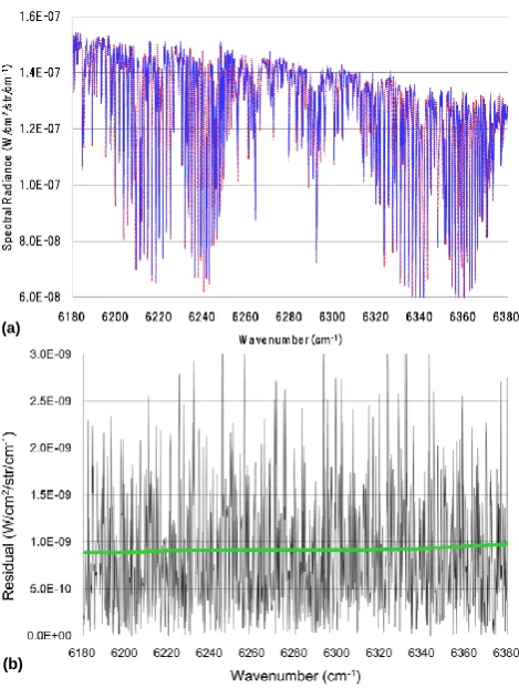
Fig. 6. (a) Measured CO₂spectrum (blue solid line) of the Level 1B V050.050 along with the modeled spectrum for the retrieval (red dotted line) and (b) the residual difference (black solid line) together with the noise level (bold green line) (courtesy of Y. Yoshida of NIES).

from the pointing mirror surface, which is estimated from the temperature telemetry data near the pointing mirror.1Bbg(ν)

is the background radiation change between BB and DS cal-ibrations, which is estimated from the orbit phase temper-ature variation model.Bobscorrected(ν) is the final Level 1B

TIR products. A more general formulation is described in Mueller matrix in Sect. 3.5.

2.7 Time data in Level 1B product

The time stamp of the telemetry data is the turnaround com-pletion timeTTAT, which corresponds to the start of

interfer-ogram acquisition. The interferinterfer-ogram near ZPD is the most informative and ZPD passing time is calculated using the fol-lowing relationship:

TZPD=TTAT+TS

XZPD

76336, (7)

whereTS is the scan duration andXzpd is the ZPD position

(10)

3 TANSO-FTS on orbit characterization and calibrations

The overall radiometric and spectroscopic performances are good and they are well within design objectives. Fig-ure 6 shows the measFig-ured CO2 spectrum of the Level 1B

V050.050 along with the modeled spectrum for the retrieval V01.10 and the residual difference (Yoshida et al., 2011). The residual is close to the noise level and the spectral resolution is as designed. In this section, the calibrations after launch are described. The instrument model and the items, which need corrections, are summarized in Tables 2 and 3, respectively. The calibration events in chronologi-cal order were described in Kuze et al. (2011b). The time-dependent degradation of the TANSO-FTS throughput (re-sponse) can be cross-checked by the methods described in the following subsections.

3.1 Radiometric calibration and on-orbit degradation

There are several ways for TANSO-FTS to estimate the cal-ibration accuracy and degradation on orbit. SWIR and TIR are calibrated independently.

3.1.1 Prelaunch calibration

As described in detail in Kuze et al. (2009) and Sakuma et al. (2010), the TANSO radiometric response was calibrated before launch by using integrating spheres. An example of the radiance conversion factor is shown in Fig. 7. TANSO-FTS has channeling in Band 2S, which is caused by multiple reflections at the band separation optics, and its magnitude is stable. As demonstrated in Fig. 7, a small oscillation feature of the conversion factor corrects channeling simultaneously and produces channeling-corrected spectral radiance. To cor-rect atmospheric absorption in the laboratory and draw the envelope, we used the thermal vacuum chamber test results that are not affected by absorption. An absolute radiometric accuracy of better than±5 % was achieved prior to launch in order to achieve better than 1 %XCO2accuracy.

3.1.2 Vicarious calibration for SWIR

The first vicarious calibration was performed in the sum-mer of 2009. The measurement campaign was conducted us-ing a dry lakebed in Railroad Valley (RRV), Nevada, USA with the NASA Atmospheric CO2Observations from Space

(ACOS) team (Kuze et al., 2011a). The spectral radiance was calibrated by comparing the satellite-measured radi-ances and simulated radiradi-ances at the top of the atmosphere (TOA). The observations at RRV suggest that the respon-sivities have changed by−9±7 %,−1±7 % and−4±7 % for bands 1, 2, and 3, respectively, from the values corre-sponding to prelaunch calibration. In 2010 and 2011, the second and third campaigns were performed and the accu-racy was improved by more frequent calibration of the

sur-Page 9/20

Fig.7. Radiance conversion factors from the Level 1B data to the spectral

radiance for the TANSO-FTS Band 2P (bold gray line) and 2S(solid line) of high

gain.

Contact

[email protected]

Germany

Fig. 7. Radiance conversion factors from the Level 1B data to the spectral radiance for the TANSO-FTS Band 2P (bold gray line) and 2S (solid line) of high gain.

face albedo measurements (Kuze et al., 2011d, 2012). As shown in Table 4a, the changes became slower 18 months after launch. The Airborne Visible/InfraRed Imaging Spec-trometer (AVIRIS) on ER-2 aircraft had flown over RRV twice at the time of GOSAT overpass on 9 October 2009 and 20 June 2011. Cross-calibrations between AVIRIS and GOSAT independently corroborated the vicarious calibration results and showed a similar trend of the degradation. Further analysis is needed for AVIRIS data.

3.1.3 Solar calibration for SWIR

(11)

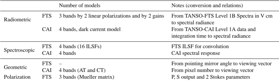
Table 2. TANSO-FTS and CAI models.

Number of models Notes (conversion and relations)

Radiometric FTS 3 bands by 2 linear polarizations and by 2 gains From TANSO-FTS Level 1B Spectra in V cm

to spectral radiance

CAI 4 bands, dark current model From TANSO-CAI Level 1A data and

integration time to spectral radiance

Spectroscopic FTS 4 bands (16 ILSFs) FTS ILSF for convolution

CAI 4 bands CAI spectral response

Geometric FTS – From pointing mirror angle to viewing vector

CAI 4 bands (AT and CT) From pixel number to viewing vector

Polarization FTS 3 bands (Mueller matrix) P, S output and 2 Stokes parameters

Table 3. TANSO-FTS and CAI correction factors.

Number of models Functions

Radiometric FTS 3 bands by 2 Linear polarizations Days from launch

CAI 4 bands Days from launch

Spectroscopic FTS Common value for all 4 bands Days from launch

Geometric FTS – Combination of AT and CT angels

campaigns. The degradation between June 2009, 2010, and 2011 is summarized in Table 4b and c.

3.1.4 SWIR trend over the Sahara desert

The Sahara and Arabian deserts are virtually clear all year round with almost no vegetation and water. We picked sev-eral sites as shown in Fig. 9a. The surface is not always Lambertian and the reflectance is dependent on the solar zenith angle. To estimate the degradation accurately, data from the same time of the year have to be compared. To minimize the random noise, several data in the same sea-son are selected and averaged. Since August, 2010, we have used the 3-point cross-track scan mode as the nominal one. Earlier measurements were made primarily in the 5-point cross-track scan mode. We compared June and July of 2009 and 2010 data using the 5-point cross-track scan mode and 2011 data using the 3-point cross-track scan mode. TANSO-FTS TIR data between 898 cm−1 and 929 cm−1 was used for cloud screening. If the maximum brightness tempera-ture is lower than 292.5K, we then assume that the data is cloud-contaminated . This screening process is applied only for the Sahara desert trend analysis. We recorded the spectral radiances of 12 971.027 cm−1_{, 6008.327 cm}−1_{, and}

4806.9806 cm−1_{in the analysis for bands 1, 2, and 3.}

Fig-ure 9b shows the degradation of the TANSO-FTS through-put for the 5 sites in one year. The change in one year was derived from a weighted average of the data over the sites, respectively, on the basis of the assumption that the aerosol optical thicknesses are the same. Since we cannot compare Sahara 8 and 9 sites, shown in Fig. 9a from the 3-point cross-track scan mode, we compared the data for June 2009, 2010

and 2011 at 3 sites instead. The results are summarized in Table 4b and c.

3.1.5 SWIR degradation estimation and correction

Even thoughXCO2 andXCH4are retrieved by using

(12)

Table 4. Estimated degradations of radiometric responsivity for TANSO-FTS and CAI from four independent methods: (a) difference from prelaunch value and initial on-orbit calibration: degradation in one year (relative): (b) between June 2009 and June 2010 and (c) between June 2010 and June 2011. Sahara Desert includes July data.

(a)

TANSO-FTS TANSO-CAI

B1 B2 B3 B1 B2 B3 B4

Vicarious calibration

June 2009 −11 % −1 % −3 % −17 % +4 % 0 % −18 %

June 2010 −14 % −2 % −5 % −20 % −3 % −4 % −19 %

June 2011 −14 % −4 % −6 % −22 % −7 % −6 % −20 %

(b)

Between June 2009 and June 2010 TANSO-FTS TANSO-CAI

B1 B2 B3 B1 B2 B3 B4

Vicarious calibration −3 % −1 % −2 % −3 % −7 % −4 % −1 %

Solar diffuser plate −2.4 % −0.7 % 0.0 % N/A N/A N/A N/A

Sahara Desert −2.0 % +0.2 % −0.2 % −1.7 % −3.9 % −0.7 % −0.3 %

Average of bands P and S

(c)

Between June 2010 and June 2011 TANSO-FTS TANSO-CAI

B1 B2 B3 B1 B2 B3 B4

Vicarious calibration 0 % −2 % −1 % −2 % −4 % −2 % −1 %

Solar diffuser plate −0.6 % −0.2 % +0.1 % N/A N/A N/A N/A

Sahara desert −0.9 % −0.5 % −0.2 % +0.2 % −1.3 % −0.4 % −0.6 %

Average of bands P and S.

the integrating sphere used for the prelaunch calibration. The gradual degradation may be attributed to contamination or changes in modulation efficiency. The upper part of Fig. 1 shows the schematics of the TANSO-FTS optics module. CAM is mounted between the pointing mirror and FTS-mechanism. CAM data over the Sahara has shown no sig-nificant degradation since launch. The possible degradation may occur in modulation efficiency of the FTS mechanism or the aft optics optical efficiency.

Lunar calibration has been performed twice a year since launch, on 11 March and 9 April 2009, 28 April and 6 June 2010, and 18 April and 14 July 2011. The bidirec-tional reflectance distribution function (BRDF) for the lu-nar surface is not Lambertian and a complicated calibration is needed for absolute calibration. These data can be used for both TANSO-FTS and CAI absolute radiometric calibra-tion. However, the lunar surface has a strong BRDF when the incident angle is zero. After the BRDF correction, the analytical results of TANSO-CAI show a similar trend, but further investigations and BRDF corrections are needed. In case of TANSO-FTS, the size of the moon disk viewed from the GOSAT orbit is about half of the instantaneous field of view (IFOV) making the analysis more complicated.

On the basis of the vicarious absolute calibration, response correction factors have been derived as a function of time (days from launch). By combining the prelaunch radiance conversion factor and these correction factors, the calibrated spectral radiance thus can be calculated. Because the surface reflectance over RRV and the solar diffuser reflectivity are high, the interferograms are calibrated with the medium gain to avoid saturation. High gain response over the Australian desert can be compared by observing the same site with high and medium gains. The ratio between the high and medium gains is determined by the feedback resistance of the ampli-fier. The comparison over the Australian desert indicated that the ratio is as designed. Thus, response correction factors de-rived from the medium gain can be applied to the high gain data. Low gain has never been used since launch.

3.1.6 Cross-calibration and validation for TIR

(13)

(a)

(b)

Fig. 8. Solar irradiance monthly calibration data from the onboard Spectralon diffuser, which indicates the change from the first mea-surement in space after correction for the distance between the satel-lite and the Sun and the angle of incidence of the solar beam upon the diffuser. The vertical lines represent the time of the 2009, 2010 and 2011 vicarious campaigns: (a) ratio of the front side radiance to the back side and (b) back side calibration.

overpasses of Infrared Atmospheric Sounding Interferometer (IASI). IASI data can be found within 100 km of the GOSAT field of view and within 10◦ of nadir. The difference in brightness temperature between 200 K and 270 K is smaller than ±1 K (Knuteson, private communication, 28 Febru-ary 2011). In addition, TIR vicarious calibration was per-formed at RRV in June 2011 by measuring surface tempera-ture and emissivity by Atmospheric Emitted Radiance Inter-ferometer (AERI) FTS together with upward spectral radia-tion by using the airborne Scanning High-resoluradia-tion Interfer-ometer Sounder (S-HIS) FTS (Tobin et al., 2006; Kuze et al., 2011d). For an atmospheric window region around 10 µm, where the radiation from the surface is dominant, it is very difficult for IASI and GOSAT to view exactly the same lo-cation at the same time. The S-HIS data covered the entire IFOV of the TANSO-FTS and the target surface temperature of RRV is 320 K. However, we cannot compare the radiation from the atmosphere above the S-HIS flight altitude. Only satellite data can provide the thermal radiation spectra from the upper atmosphere where the radiation from the surface is fully absorbed. A combination of formation flight of a high-altitude (20 km) aircraft and match-up data from other

satel-(a)

(b)

Fig. 9. (a) Radiance monitoring sites over the Sahara and Arabian deserts. (b) TANSO-FTS degradation in one year between 2009 and 2010 over the Sahara desert.

lites can calibrate the wide range of spectral radiance from both atmosphere and ground surface. Both cross-calibrations with IASI and S-HIS agree well within±1 K. These data are still being analyzed and compared.

3.2 Signal-to-noise ratio

There is no stable onboard white light source available for radiometric calibration purposes to estimate the noise level along with a known signal level. Therefore, SNR cannot be measured explicitly. It is estimated from the imaginary spec-tra or out-of-band real specspec-tra. Currently the noise level is the same as measured before launch. There is no signifi-cant response degradation. Thus, we can expect the SNR performance to be reasonably similar to that described by Kuze et al. (2009). There are two dominant noise sources for TANSO-FTS bands 1, 2, and 3. One is the detector and its electronics noise, which is independent of the input sig-nal level and proportiosig-nal to the square root of the electric band width. The performance can be measured with dark in-put data and can be expressed with specific detectivity (D*). The second source is the shot noise, which is proportional to the square root of the total number of input photons. Band 2 has wide optical band width of 5800–6400 cm−1to cover CO2, CH4and H2O lines, here the shot noise contribution is

(14)

3.3 Spectral resolution and instrument line shape function

3.3.1 Prelaunch calibration and simulated model

The geophysical parameters are retrieved by comparing the measured spectral radiance and the simulated radiance at the top of the atmosphere.XCO2,XCH4, and other

geophys-ical parameters such as surface pressure can be retrieved by minimizing the residual between the measured spectrum and simulated spectrum convolved with the instrument line shape function (ILSF). Because ILSF is a function of the wavelength, ILSFs at selected wavelengths are modeled as shown in Fig. 10a. The models are simulated because the prelaunch tests with monochromatic light from tunable diode lasers were performed at limited wavenumbers and did not cover the whole spectral range. Off-axis mounting of the de-tector due to imperfect alignment creates an asymmetry of ILSF; however, this effect can be numerically simulated. The ILSF at short wavelengths is more sensitive to the misalign-ment, thus the detector position during the integration has to be accurately measured. Misalignment from the ideal opti-cal axis of the Band 1P and 1S are estimated by introduc-ing monochromatic light from tunable diode lasers prior to launch. Spatial uniformity over the scene aperture and angu-lar uniformity over the entire IFOV are particuangu-larly important for this characterization. Although the prelaunch test config-uration was imperfect, the data nevertheless contains detec-tor offset information. By carefully simulating the imperfect prelaunch test configuration, the offset value was estimated. The best estimate ILSF models were calculated using the off-set value and optical aberration. On the other hand, for bands 2, 3, and 4, ILSF are much less sensitive to the misalign-ment of the detector, and being less than 50 µm, the finite size effect of IFOV has been considered.

3.3.2 Spectral resolution on orbit

Figure 10b shows the long term stability of the data using the onboard ILSF calibration laser which has 6460 cm−1 frequency. Although the frequency of the onboard diode laser without temperature control is not constant and the laser cannot illuminate the solar diffuser plate uniformly, the ILSF shape itself has been very stable since launch; this indicates that no significant spectral resolution change has been observed.

3.3.3 Absolute spectral calibration

By carefully monitoring sampling laser output level of the FTS mechanism and the solar Fraunhofer line positions, we have observed a gradual decrease of the laser signal detec-tion level and an increase of the apparent wavenumber of the Fraunhofer lines. The degradation of laser signal detection level is exponential and smaller than 10 % in one year and is slowing down. We estimate that the laser will still have a

(a)

(b)

Fig. 10. (a) ILSF models at typical wavelength of each spectral

band: 13 050 cm−1of Band 1P (bold gray), 6025 cm−1 of Band 2

(dash-dotted), 5000 cm−1of Band 3 (solid) and 700 cm−1of Band

4 (dotted). (b) Overwritten ILSF acquired monthly on orbit from March 2009 to April 2010 using the onboard diode laser which has

6460 cm−1frequency.

sufficient level of control after 10 years of operation. We con-sider that the laser signal detection level decrease and the ap-parent increase in Fraunhofer wavenumbers are related. Be-cause all bands have the same spectral calibration factors, the most probable cause is a change in optical alignment of the laser beam on orbit as illustrated in Fig. 11. As a con-sequence, the illumination on the laser detector has become weaker, maximum OPD has become larger, and spectral res-olution has become slightly higher. The absolute spectral po-sition can be calibrated by applying the spectral correction factor with time:

νcorre=νraw/ (a0exp(a1t )+a2), (8)

whereνcorre, νraware wavenumbers before and after the

cor-rection, anda0,a1,a2, andt are the calibration coefficients

and time from launch. As shown in Fig. 12, the change since launch is less than 10 ppm and the effect on spectral resolution is negligibly small.

3.4 Geolocation and pointing characterization

(15)

Page 14/20

Fig.11. Schematics of the sampling laser misalignment and OPD.

Bahnhofsallee 1e

Contact

[email protected]

Germany

Based in Göttingen Registered in HRB 131 298 County Court Göttingen Tax Office FA Göttingen USt-IdNr. DE216566440 Fig. 11. Schematics of the sampling laser misalignment and OPD.

the ground. The resolvers are sensitive to their electromag-netic environment and are suspected to have errors, which are of two kinds. One kind of error is a known offset (pre-dictable) that the onboard resolver can detect and that the Level 1B process can correct. The other is an unpredictable error, which the resolver cannot detect. The error is a possible resolver anomaly most likely due to noise induced by elec-tromagnetic interference. The second error was first detected just three months after launch (April 2009) and had not been stable until August 2009. To estimate the offset values, we use images acquired with the Advanced Visible and Near In-frared Radiometer type 2 (AVNIR-2) on the Advanced Land Observing Satellite (ALOS) (Tadono et. al., 2009) and CAM data of the ground correction points (GCP). There is no gen-eral formula to express the pointing error. Instead we have been providing the offset information since September 2009 and an example is shown in Table 5. Offset values have slowly changed with time. It is a function of the scanning pattern and not of other considerations, such as the location on Earth. Regarding the pointing error, settling down (over-shoot) is not ideal when the AT range of motion is large. The offset level is not a simple linear function of AT and CT an-gles. Hence, the geometrical correction in the 3-point cross-track scan mode is not the same as that in the target mode and the 5-point cross-track scan mode.

3.5 Polarimetric calibration by Mueller matrix

Both instrument and scene flux scattered by the Earth’s at-mosphere have large polarization. The protection coating on the silver pointing mirror surface has a polarization phase. To calculate the response to the polarized input scene flux, the polarization reflectivity and phase of the instrument need to be considered. The relation between input flux Stokes vec-tor and two linear polarizations “P“ and “S“ of TANSO-FTS measurements can be expressed using the Mueller matrix as follows:

SPoutput=MppMoptMr(−θCT)Mp(θAT)Mm(θAT)

Mr(θCT) Sinput, (9)

Page 14/20

Fig.11. Schematics of the sampling laser misalignment and OPD.

Bahnhofsallee 1e

Contact

[email protected]

Legal Body

Copernicus Gesellschaft mbH

37081 Göttingen Germany

http://publications.copernicus.org Phone +49-551-900339-50

Fax +49-551-900339-70

Based in Göttingen Registered in HRB 131 298

County Court Göttingen

Tax Office FA Göttingen USt-IdNr. DE216566440

Fig. 12. Spectral calibration factor as a function of days from launch.

SSoutput=MpsMoptMr(−θCT)Mp(θAT)

Mm(θAT)Mr(θCT) Sinput, (10)

where Mpp,Mps,Mopt,Mp,Mm, and Mr are Mueller

ma-trixes of polarization beam splitter, optical efficiency of the FTS-mechanism and aft optics, phase difference due to the pointing mirror surface coating, pointing mirror reflec-tivity, and CT rotation, respectively.SPoutput,SSoutput,Sinput, θCT, and θAT are output and input signals of the Stokes

vector and the CT and AT angles, respectively. Sinput, the

Stokes vector at the top of the atmosphere, can be calcu-lated with a vector radiative transfer model. By comparing the simulatedI components of the Stokes vectorSPoutput and SSoutput(IPopCandISopC)andIPopMandISopMmeasured

spec-tral radiance with TANSO-FTS,XCO2 andXCH4 can be

in-dependently retrieved from SWIR P and S bands. The ref-erence plane for polarization for the input Stokes vector, of which components are I, Q, U, and V, is defined by the local normal at the target and the ray from the target to the satellite. The prelaunch radiometric calibration was performed on the ground by introducing un-polarized light from nadir, of which input and output spectral radiance are

IipPL, IPopPL and ISopPL, respectively. The prelaunch

cali-bration data with the Level 1 format can be expressed in

RP IPopPL and RS ISopPL. The radiance conversion

ta-ble prepared prelaunch shows the relation between IipPL,

RP IPopPL, andRS ISopPLas shown in Fig. 7.IPopPLand

ISopPLare not used explicitly in radiometric calibration.

The above mentioned Mueller matrix needs to be used to correct the AT and CT angle dependency of the pointing mir-ror in the case of slant looking. Thus the correction requires the pointing mirror reflectivity and phase information in Mp

and Mm as the function of AT angle (the incident angle to

(16)

Table 5. TANSO-FTS pointing onboard anomaly and correction: upper table is for the 5-point cross-track mode scan and lower one is for the 3-point cross-track scan mode. IDs in the tables are illustrated in Fig. 2. These are typical values and the offsets have changed with time.

(a) 5-point cross-track scan mode

ID AT (km) Direction CT (km) Direction

0 8.3 positive down track * 2.1 the left of the ground track **

1 −0.5 negative down track −0.4

the right of the ground track

2 0.0 positive down track −0.6

3 −0.7

negative down track −0.6

4 −0.1 −0.4

5 9.2

positive down track 2.0 the left of the ground track

6 0.7 −0.1 the right of the ground track*

7 -0.3

negative down track

−0.3

the right of the ground track

8 −1.1 −0.4

9 −1.3 −0.5

(b) 3-point cross-track scan mode (typical values)

ID AT (km) Direction CT (km) Direction

0 5.0

positive down track

3.0

the left of the ground track

1 5.1 3.0

2 5.4 3.2

3 5.2 2.6

4 5.2 2.8

5 5.2 2.8

6 5.7 3.5

7 6.1 3.7

8 5.8 3.6

9 6.0 3.0

10 5.9 3.0

11 5.8 3.0

12 6.2 2.9

13 6.2 3.0

14 6.2 3.0

15 5.0 3.5

16 5.0 3.6

17 5.6 3.7

* Forward looking=looking south-southwest at the equator for the descending track (dayside). ** Left of the ground track=the east-southeast at the Equator for the descending track (dayside).

individual optical efficiency is not needed for the radiometric calibration for the on-orbit data. This coating has been opti-mized for the SWIR region with higher than 99 % reflectivity and the AT angle dependency of SWIR bands is very small.

However, the reflectivity is lower and the polarization sensitivity is higher in some TIR wavelength, as shown in Fig. 14b. As discussed in Sect. 2.6, measured spectral radi-anceSToutputcan be expressed using the scene fluxSTinput,

ther-mal radiation from the pointing mirror, and the background radiation in the following Mueller matrix:

SToutput=MoptMr(−θCT)Mm(θAT)Mr(θCT) STinput

+MoptMr(−θCT)Me(θAT) STmirror+1SBG, (11)

where Me, STmirror, and1SBG are Mueller matrix of

point-ing mirror emissivity, Stokes vectors of the radiation from the pointing mirror, and the background radiation variation

between calibrations, respectively.I component ofSTinput is

retrieved from Eq. (11) in the TIR Level 1 processing. 3.6 Quality flag of data products

(17)

(a)

(b)

Fig. 13. Measured phase of the pointing mirror using the witness sample for Mueller matrix of incident angles of 35, 40, 45, 50 and 55 deg: (a) Band 1 and (b) bands 2 and 3.

stability on orbit has so far been much better than 1 % and so the speed-instability flag has not yet been triggered.

3.7 Additional corrections

Methods of conversion, calibration and correction are de-scribed in this paper. The Level 1 products and calibration data include all the information required to produce Level 2 products. In parallel, for the detailed Level 1 product analy-sis, additional software corrections are applied as follows:

(i) Finite size of the field of view; finite size of the field of view has a self-apodization effect. Without large degra-dation of the spectral shape, the self-apodization due to the size is corrected as described by Knuteson et al. (2004). Only Band 4 data can be additionally cor-rected for meteorological application.

(ii) Wavelength shift correction; the shift due to the opti-cal alignment change of the sampling laser is corrected even though the value of the shift since launch is small enough.

(iii) Mueller matrix; four-by-four elements for 3 TANSO-FTS SWIR bands are added to the Level 1 data.

(a)

(b)

Fig. 14. Measured spectral reflectivity of the pointing mirror using the witness sample for two linear polarizations (P and S) of the in-cident angles of 35, 45, and 55 deg: (a) SWIR and (b) TIR.

(iv) Geometric correction; the most probable offset correc-tion of the pointing mirror estimated from CAM data is applied.

(v) Spectral radiance conversion; the Level 1 data having units of V cm are converted to the calibrated spectral radiance having units of W cm−1_str−1_.

4 TANSO-CAI Level 1A data processing, characterization, and calibration

The design and prelaunch performance and calibration of TANSO-CAI were described in detail in Kuze et al. (2009). The TANSO-CAI Level 1A data processing, on-orbit perfor-mance, and calibration are described in this section. Instru-ment models and calibrations are summarized in Tables 2 and 3. JAXA has been providing the raw Level 1 data to NIES and other users. In this section, we describe how to correct the raw data and convert it to spectral radiance.

4.1 Radiometric calibration and correction

(18)

Table 6. Sampling interval non-uniformity as a function of OPD of the forward and backward scans.

Source Item Criteria

Satellite Orbit control Data acquired during orbit control

FTS

Saturation Interferogram saturation, Blackbody temperature

Spike Fluctuation, Cosmic ray

Low frequency disturbance (jitter) Satellite and point mechanism microvibration

Pointing error AT and CT pointing error larger than 0.1deg

FTS mechanism temperature Lower than 20◦or higher than 26◦

Large ZPD position shift Shift larger than 100 laser fringes

Scan speed instability FTS scan speed instability larger than 2 %

4.1.1 Offset subtraction and spectral radiance conversion

The TANSO-CAI Level 1A data includes signals and off-sets which vary depending on the total input radiance, and dark currents. The observed spectral radiance is calculated by extracting the offset and dark current using the following equation:

Sobs(n)=

VC(n)−VCpre−VC dark(n, Tint)

TintRC(n)

, (12)

whereVC(n),VCdark(n), and RC(n) are output, dark level,

and response of the pixel number n, respectively.Tintis the

integration time of the detectors.VCpreis the average of

out-put of the first three prescan pixels and calculated separately for the odd and the even pixels. We assume that the dark level is a function of the integration time and is constant with time since launch.RC(n)is based on the prelaunch calibration and

degradation correction is described below. 4.1.2 Pixel-to-pixel non-uniformity correction

All the pixels of each band were calibrated at the same time before launch by using the integrating sphere, the inner sur-face of which is coated with barium sulfate (BaSO4).

Radia-tion emanating from the aperture of the integrating sphere has a non-Lambertian angular distribution, especially for bands 1 (UV) and 4 (SWIR). Spectral radiance of the inte-grating sphere was calibrated at a direction perpendicular to the aperture and its angular distribution was not calibrated before launch. As TANSO-CAI has a wide field of view, the prelaunch data other than the center pixel has to be corrected as follows. The telescope optics of bands 1 and 4 have very small vignetting while bands 2 and 3 have large vignetting. Therefore, the angular distribution of bands 1 and 4 can be corrected. To check pixel-to-pixel uniformity, we assume the averaged Earth albedo is uniform when TANSO-CAI data ac-quired from all the 44 paths over one year. The Earth albedo is defined as the measured reflectance at the top of the at-mosphere. By correcting Rayleigh scattering and sun glint effect, pixel-to-pixel non-uniformity can be detected and cor-rected using the averaged measured data for Band 1. There

Page 19/20

Fig.15. Radiance conversion factorsfor the TANSO-CAI Band 1.

Contact

[email protected]

Germany

Fig. 15. Radiance conversion factors for the TANSO-CAI Band 1.

was no need for pixel-to-pixel correction for Band 2. For Band 3, local bump structures are corrected using one-year averaged data. Band 4 is corrected using one-year averaged data, except for several pixels, of which dark current have increased. Pixel 154 shows the sudden increase after pass-ing through the South Atlantic Anomaly. The data shown in Fig. 15 is the pixel-to-pixel non-uniformity correction of Band 1. These corrected radiance conversion factors are used for the TANSO-CAI Level 1B product.

4.1.3 Degradation after launch