www.nonlin-processes-geophys.net/21/19/2014/ doi:10.5194/npg-21-19-2014
© Author(s) 2014. CC Attribution 3.0 License.
Nonlinear Processes
in Geophysics
Representation of model error in a convective-scale ensemble
prediction system
L. H. Baker, A. C. Rudd, S. Migliorini, and R. N. Bannister
Department of Meteorology, University of Reading, Earley Gate, P.O. Box 243, Reading, RG6 6BB, UK
Correspondence to: L. H. Baker ([email protected])
Received: 27 June 2013 – Revised: 29 November 2013 – Accepted: 10 December 2013 – Published: 8 January 2014
Abstract. In this paper ensembles of forecasts (of up to six hours) are studied from a convection-permitting model with a representation of model error due to unresolved processes. The ensemble prediction system (EPS) used is an experimen-tal convection-permitting version of the UK Met Office’s 24-member Global and Regional Ensemble Prediction System (MOGREPS). The method of representing model error vari-ability, which perturbs parameters within the model’s param-eterisation schemes, has been modified and we investigate the impact of applying this scheme in different ways. These are: a control ensemble where all ensemble members have the same parameter values; an ensemble where the param-eters are different between members, but fixed in time; and ensembles where the parameters are updated randomly ev-ery 30 or 60 min. The choice of parameters and their ranges of variability have been determined from expert opinion and parameter sensitivity tests. A case of frontal rain over the southern UK has been chosen, which has a multi-banded rainfall structure.
The consequences of including model error variability in the case studied are mixed and are summarised as follows. The multiple banding, evident in the radar, is not captured for any single member. However, the single band is posi-tioned in some members where a secondary band is present in the radar. This is found for all ensembles studied. Adding model error variability with fixed parameters in time does increase the ensemble spread for near-surface variables like wind and temperature, but can actually decrease the spread of the rainfall. Perturbing the parameters periodically through-out the forecast does not further increase the spread and ex-hibits “jumpiness” in the spread at times when the parame-ters are perturbed. Adding model error variability gives an improvement in forecast skill after the first 2–3 h of the fore-cast for near-surface temperature and relative humidity. For
precipitation skill scores, adding model error variability has the effect of improving the skill in the first 1–2 h of the fore-cast, but then of reducing the skill after that. Complemen-tary experiments were performed where the only difference between members was the set of parameter values (i.e. no initial condition variability). The resulting spread was found to be significantly less than the spread from initial condition variability alone.
1 Introduction
Errors in forecasts originate from a number of sources, namely the initial conditions, the boundary conditions and the model formulation. In synoptic scale forecasts of lead times up to a day, it is thought that the first two sources dom-inate. However, at convective scale model errors are thought to become more important, especially for relatively short range forecasts. Here we investigate a proposed representa-tion of model error that can influence the forecast skill at con-vective scale. We use an experimental convection-permitting version of the UK Met Office’s 24-member Global and Regional Ensemble Prediction System (EPS) (MOGREPS) (Bowler et al., 2008): the southern UK 1.5 km EPS (Miglior-ini et al., 2011; Caron, 2013). We focus on the effect of model error resulting from the parameterisation of unre-solved processes; specifically microphysics and turbulent boundary layer processes. In this study we modify the so-called Random Parameters (RP) scheme, used in MOGREPS (Bowler et al., 2008), by applying changes designed to make it appropriate for use in a convective-scale ensemble.
the forecast skill. By evaluating these effects, we determine how useful this scheme could be as a method of representing model error in a convective-scale EPS. Although it is difficult to draw general conclusions from one case study, this work presents new results of the impact of a model error scheme on a convection-permitting model.
There are several different methods commonly used to rep-resent model error. In the multiphysics method (also some-times called the multimodel method), a set of different model physics parameterisation schemes is used, and generally an ensemble is constructed of members which use different combinations of schemes (Stensrud et al., 2000; Berner et al., 2011; Clark Jr. et al., 2010; Clark et al., 2011). The stochastic kinetic energy backscatter (SKEB) scheme of Shutts (2005) (developed further by Berner et al., 2009 and used by Berner et al., 2011) aims to replace upscale kinetic energy lost in the numerical integration of the model and in the parameter-isation of unresolved processes. Another method is to use a stochastically perturbed physical tendencies (SPT or SPPT) scheme (Buizza et al., 1999; Bouttier et al., 2012; Fresnay et al., 2012), in which the total tendencies from parameter-isation schemes are perturbed. A further method, and the one on which we focus here, is to perturb a set of individual parameters within the parameterisation schemes themselves. This method can be applied in two different ways: the first is to perturb individual or sets of parameters about their de-fault values, and keep these perturbed values fixed through-out each forecast; the second is to use a stochastic technique to vary the parameter values periodically throughout the forecast. The fixed parameter perturbation method has been widely used for global ensembles (notably the climatepre-diction.net multi-thousand member ensemble project (Mur-phy et al., 2004; Stainforth et al., 2005) and the Met Office’s Quantifying Uncertainty in Model Predictions (QUMP) en-semble (Murphy et al., 2004)), mesoscale enen-semble sys-tems (Hacker et al., 2011) and convection-permitting mod-els (Gebhardt et al., 2011; Vié et al., 2012). In this study we use both methods of setting parameter values (see Sect. 2.2 for details of the scheme used when updating parameters periodically). A similar method was also used by Lin and Neelin (2000) and Bright and Mullen (2002), but for only one and two parameters, respectively. The advantage of up-dating the parameters throughout the forecast is that it in-creases the amount of random variability in the parameters, and increases the volume of parameter values explored dur-ing the period of the forecast. However, a disadvantage of this method is that perturbing the parameters during the forecast may introduce jumps, loss of conservation of quantites that should be conserved, and changes of state, which may lead to undesirable effects on the forecast. For the purposes of this study, the RP scheme is a logical choice since the basic RP framework already exists in the Met Office Unified Model (MetUM), and some parameters for which there is genuine uncertainty in their values had already been identified and their uncertainty quantified. We note that this method of
rep-resenting model error is not guaranteed to increase the en-semble spread, due to the nonlinear dependence of the model on the parameters.
In Sect. 2 we describe the configuration of the MetUM, the formulation of the RP scheme and the evaluation tools used, and give an outline of the experiments performed in Sects. 4 and 5. In Sect. 3 we describe the meteorology of the case used in this study, and show results of parameter sensitivity tests performed for this case. In Sect. 4 we evaluate the per-formance of the control (no model error) ensemble, and in Sect. 5 we evaluate the effects of model error variability on the forecast skill and on the spread of the ensemble. Finally, Sect. 6 provides a summary and discussion of our results.
2 Methodology
2.1 Description of the 1.5 km EPS
This work was performed using the MetUM version 7.8. The MetUM is a finite-difference model that solves the non-hydrostatic, fully compressible, deep-atmosphere dynami-cal equations with a semi-Lagrangian, semi-implicit inte-gration scheme. The equations are solved on a horizontally staggered Arakawa C grid and a terrain-following hybrid-height vertical coordinate with Charney–Phillips grid stag-gering (Davies et al., 2005). In all the MetUM ensemble sys-tems discussed here, boundary-layer mixing is parameterised using the scheme of Lock et al. (2000) and large-scale pre-cipitation is parameterised using the scheme of Wilson and Ballard (1999). In the global and regional formulations of the ensemble system (MOGREPS-G and MOGREPS-R, respec-tively, described in more detail below), convection is parame-terised using the scheme of Gregory and Rowntree (1990); no convection scheme is used in the 1.5 km EPS. To limit the occurrence of grid-point convection in the 1.5 km EPS, a prognostic rain variable is advected with the wind field, fol-lowing Sect. 2d of Lean et al. (2008). In MOGREPS-G and MOGREPS-R, gravity-wave drag is parameterised using the scheme of Webster et al. (2003); this scheme is not active in the 1.5 km EPS.
resolution equivalent to 60 km in the mid-latitudes and the same vertical levels as MOGREPS-R1.
A 24-member ensemble is generated in MOGREPS-G us-ing an ensemble transform Kalman filter (ETKF) (Bishop et al., 2001). The ETKF is used to produce a set of per-turbations which can be added to the Met Office 4-D-Var analysis to give the initial conditions (ICs) for the ensemble members. A detailed description of the way that the ETKF is used to generate these IC perturbations is given in Bowler et al. (2008). MOGREPS-G is run with 12 h cycling2, start-ing at 00:00 UTC and 12:00 UTC. MOGREPS-R also runs with 12 h cycling starting at 06:00 UTC and 18:00 UTC, but takes its initial conditions and hourly lateral boundary con-ditions (LBCs) from MOGREPS-G. In this study we run a MOGREPS-G forecast starting at 00:00 UTC 20 Septem-ber 2011 and extend the forecast to 19:00 UTC. We use this to provide ICs and LBCs for a MOGREPS-R forecast start-ing at 06:00 UTC, which outputs hourly ICs and LBCs for the 1.5 km EPS from 07:00 UTC to 18:00 UTC.
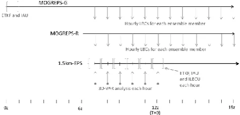
The 1.5 km EPS is described in detail by Migliorini et al. (2011). Subsequent improvements to the 1.5 km EPS setup using the so-called scale-selective ETKF to avoid ensemble perturbation mismatches between the ICs and LBCs are de-scribed by Caron (2013). In this study we run a 13 h fore-cast with hourly ETKF cycling for the first 6 h, followed by a 7 h forecast, forced by hourly LBCs from MOGREPS-R. The system is described schematically in Fig. 2. In each of the ETKF cycles, the initial conditions for the 1.5 km EPS control member are produced from a 3-D-Var analysis, with LBCs provided by a 4 km grid-spacing model with a do-main covering the whole UK. For each 1.5 km EPS ensem-ble member, a perturbation is applied to the control member ICs. These IC perturbations are derived from MOGREPS-R as follows: in the first cycle, the IC perturbations for the 1.5 km EPS ensemble members are downscaled from the MOGREPS-R IC perturbations; in subsequent cycles, the 1.5 km EPS IC perturbations are partitioned into small-scale and large-scale components. The small-scale component of the IC perturbations is derived by applying the scale-selective ETKF to the 1.5 km EPS forecast perturbations from the pre-vious cycle. The large-scale component of the 1.5 km EPS ICs is derived by using the downscaled MOGREPS-R fore-cast perturbations for each ensemble member to perturb the 1.5 km analysis. An inflation factor is applied to scale the per-turbations. This ensures that the innovation variance is con-sistent with observations atT+1 of the forecast (Migliorini et al., 2011; Caron, 2013). A spatially and temporally fixed inflation factor value is used throughout the forecast. A suit-able value for the inflation factor in the particular case stud-ied here was determined by examining power spectra of
po-1The current operational version of MOGREPS-G runs at a
higher resolution than this, with a grid length of 33 km in the mid-latitudes.
2The current operational version has 6 h cycling.
Fig. 1. Schematic diagram showing the model domains of
MOGREPS-G, MOGREPS-R and the 1.5 km EPS used here. Taken from Fig. 1 of Caron (2013).©Crown Copyright 2013, Met Office.
Fig. 2. Schematic diagram showing the model setup of the 1.5 km
EPS used in this study. Times shown are for 20 September 2011.
2.2 The random parameters scheme as a method of representing model error
The RP scheme is used operationally in MOGREPS (Bowler et al., 2008). The scheme is designed to simulate model error due to uncertainty in the parameterisation of sub-grid scale processes. The RP scheme takes a set of parameters from var-ious parameterisation schemes and treats them as stochastic variables. For each parameter, a physically sensible range of values has been defined as advised by experts. The parameter is allowed to vary within this range.
In the original RP scheme, two parameters from each of the boundary layer, large-scale precipitation, gravity-wave drag and convection schemes were selected (see Table 1 of Bowler et al. (2008) for the full list of parameters and val-ues). Five additional boundary layer parameters were later added to the RP scheme following the work of Zadra and Lock (2010). The full set of boundary layer and large-scale precipitation scheme parameters used in this updated scheme is shown in the top part of Table 1.
The parameter values are calculated first using the first-order autoregression model
Pt0=µ+r(Pt−1−µ)+, (1)
wherePt0andPt−1are the intermediate and previous
param-eter values,µ is the mean value3 of the parameter distri-bution (taken to be the default value of that parameter) and
r is the auto-correlation constant (set asr=0.95). is the stochastic shock term, sampled from a uniform distribution in the range±(Pmax−Pmin)/3, wherePmaxandPminare the
maximum and minimum values for the parameter. IfPt0is outside of the prescribed range, it is rounded down or up to give the new parameter value,Pt:
Pt=
Pmin if Pt0< Pmin, Pmax if Pt0> Pmax, Pt0 otherwise.
(2)
3µis not necessarily the true mean of the resulting distribution
of parameter values. The true mean is influenced by the rounding process described in Eq. (2).
Fig. 3. Met Office mean sea level pressure analysis charts valid at (a) 12:00 UTC and (b) 18:00 UTC 20 September 2011. Grey
pres-sure contours every 4 hPa.©Crown Copyright 2011, Met Office.
The range of and the value of r were chosen following a series of 72 h forecasts and selecting the combination of values that gave the maximum spread and best determinis-tic scores for individual ensemble members (Bowler et al., 2008). These values are therefore tuned for the resolution of MOGREPS-G, which at the time had 90 km grid spacing.
In the standard formulation of the RP scheme, the param-eters are updated using Eqs. (1) and (2) once every 3 h. The parameter values are then fixed for a period of 3 h until the next update time. The same parameter values are used for all grid points. Each time the scheme is applied, a new random numberk∈ [0,1]is generated to give a different value of
defined as=(2k−1)(Pmax−Pmin)/3. A different random
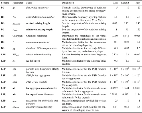
Table 1. Parameters used in the modified RP scheme. The four pairs of parameters that vary together (using the same random number to
updatein Eq. 1) are shown in their respective pairs in italics and bold. ParameterRicvaries asRic=10/g0.
Scheme Parameter Name Description Min Default Max
BL g0 flux profile parameter Controls stability dependence of turbulent
mixing coefficients in the stable boundary-layer scheme.
5 10 20
BL Ric critical Richardson number Determines the boundary-layer top (defined
as the lowest level for whichRi > Ric).
0.5 1.0 2.0
BL gmezcla neutral mixing length Sets the magnitude of the turbulent mixing lengths.
0.03 0.15 0.45
BL λmin minimum mixing length Sets the magnitude of the turbulent mixing lengths.
8 40 120
BL Charnock Charnock parameter Determines the magnitude of the wind-speed dependent roughness length over sea.
0.010 0.011 0.026
BL A1 entrainment parameter Multiplication factor for the entrainment rate at the boundary-layer top.
0.1 0.23 0.4
BL g1 cloud-top diffusion parameter Multiplication factor for the eddy diffusiv-ity at the cloud top in the boundary layer.
0.5 0.85 1.5
LSP RHcrit critical relative humidity Relative humidity at which cloud begins to form.
0.875 0.9 0.910
LSP mci ice-fall speed Multiplication factor for the fall speed of ice crystals.
0.3 1.0 3.0
LSP x1r particle size distribution (PSD) for rain
Multiplication factor for the PSD function for rain.
2×10⁶ 8×10⁶ 2×109
LSP x1i PSD for ice aggregates Multiplication factor for the PSD function
for ice aggregates.
1×10⁶ 2×10⁶ 1×107
LSP x1ic PSD for ice crystals Multiplication factor for the PSD function
for ice crystals.
1×10⁷ 4×10⁷ 1×10⁸ LSP ai ice aggregate mass diameter Multiplication factor for the mass–diameter
relationship for ice aggregates.
0.0222 0.0444 0.0888
LSP aic ice crystal mass diameter Multiplication factor for the mass–diameter relationship for ice crystals.
0.2935 0.587 1.174
LSP tnuc maximum ice nucleation tem-perature
Maximum temperature at which ice crystals can form.
−25 −10 −1 LSP ecauto autoconversion efficiency Collection/collision coefficient for the
con-version of cloud liquid water to rain.
0.01 0.55 0.6
control member, is given a different set of random parameter perturbations by the RP scheme.
2.3 Modifications to the scheme for the convective-scale EPS
To apply the RP scheme to a forecast ensemble run in the 1.5 km EPS convective-scale setup, it was necessary to make some modifications to the existing scheme. Importantly, at this resolution, the convection scheme and gravity-wave drag schemes are not used. Therefore, only parameters in the boundary layer and large-scale precipitation schemes were perturbed. Sensitivity tests were used to determine appropri-ate parameters in the large-scale precipitation scheme to per-turb. These tests are described in Sect. 3.3. The full set of parameters used here is given in Table 1.
Given the shorter time step of the high-resolution forecast compared with the global and NAE forecasts (50 s compared with 5–10 min) and the short forecast lead times we are in-terested in, it was appropriate to revise the time interval be-tween calls to the RP scheme (3 h in the original scheme). We test update times of 30 and 60 min, which were chosen to allow the parameters to vary smoothly over time, without giving continual shocks to the model. Consideration was also given to the timescales of the processes that the parameterisa-tion schemes represent. A further version of the RP scheme, holding parameters fixed throughout the forecasts, was also used. In all cases the first application of the RP scheme is at
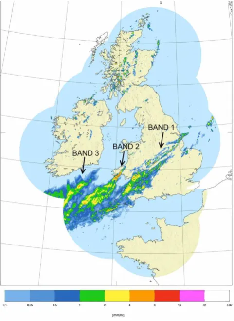
Fig. 4. Radar-derived surface precipitation rate (1 km composite)
at 15:00 UTC 20 September 2011.©Crown Copyright 2011, Met Office.
2.4 Evaluation and verification methods
We evaluate the spread and skill of the ensemble by con-sidering near-surface fields (1.5 m temperature, 1.5 m rela-tive humidity (RH) and 10 m wind speed), rainfall rate and rainfall accumulation. These quantities were chosen because they could be evaluated against surface and radar observa-tions that were available to us.
To evaluate the spread of the ensemble we use two differ-ent diagnostics: the first is a domain-averaged measure of the ensemble spread at each time; the second, for the hourly rain accumulation only, is the correspondence ratio (CR), which gives a measure of spread for a whole field rather than in-dividual grid points (as used by Gebhardt et al., 2011). We define the spread for ann-member ensemble as
spread= 1
nx×ny
nx,ny X
i,j=1 σi,j,
where
σi,j= v u u t
1
n−1
n X
k=1
(pi,j,k−pi,j)2,
nxandnyare the numbers of grid points in thex andy di-rections, respectively (in our casenx=360 andny=288),
pi,j,k denotes the value of fieldp at point(i, j )for
ensem-ble memberkandpi,j is the ensemble mean value of field
pat point(i, j ). CR is calculated following Gebhardt et al. (2011) as CR=N (Pall)/N (P≥1), whereN (Pall)is the
num-ber of grid points where all memnum-bers forecast an event, and
N (P≥1)is the number of grid points where at least one
mem-ber forecasts the event. A low CR indicates large ensemble spread, while a high CR value indicates that the ensemble members are generally in agreement.
To evaluate the forecast skill of the ensemble by compar-ing with observations, we use three methods: the first, for rain and near-surface fields, is the continuous ranked probability score (CRPS); the second, for rainfall accumulation only, is the precipitation skill score (PSS); the third, for rainfall rate only, is the innovation magnitude.
The CRPS is a way of measuring the closeness between two cumulative distribution functions (CDFs). In our case the two CDFs are those of a forecast,Ff(x), and of an observa-tion,Fo(x). The definition of the CRPS at point(i, j )and for quantityxi,jis the total squared difference between these
CDFs: CRPSi,j =
∞ Z
xi,j=−∞
dxi,j(Ff(xi,j)−Fo(xi,j))2,
(Wilks, 2006), where the CDFs are Ff/o(xi,j)= Rxi,j
xi,j0 =−∞dx 0
i,jPf/o(xi,j0 )and where Pf/o(xi,j)is the
proba-bility density function (PDF) for the forecast/observation at the point(i, j ). The forecast’s PDF is described by the ensemble members, xi,j(k), by assuming that each is equally likely:Pf(xi,j)=PNi=1δ(xi,j−xi,j(k)), whereδ is the Dirac
delta-function. In previous works using the CRPS, an obser-vation’s PDF assumes that the observation is perfect, i.e. that
Po(xi,j)=δ(xi,j−yi,jo ), where yi,jo is the observed value,
which leads to the observation’s CDF being a Heaviside step function. This simplifies the calculation of the CRPS as it avoids the need to do explicit quadrature (see Sect. 4 of Hersbach, 2000). In this work though we account for imperfect observations by assuming that each observation’s PDFs is a normal distribution with finite width,σo. In this
case the CRPS reduces to the following calculation:
CRPSi,j = ∞ Z
xi,j=−∞
dxi,j
1
Nnf(xi,j)−
1 2
"
1+erf xi,j
−yi,jo
√
2σo
!#)2
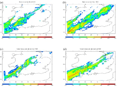
Fig. 5. Observed and model rain rate (mm h−1). Left column: 15:00 UTC (T+3), right column: 18:00 UTC (T+6) 20 September 2011. Top row: radar-derived surface precipitation rates (1 km composite), bottom row: control forecast rainfall rate at the surface.
wherenf(xi,j)is the number of ensemble members whose
forecast values are less than or equal toxi,j and erf(x)is the
standard error function erf(x)=√2 π
Rx
x0=0exp−x2dx. Nu-merical quadrature is necessary to evaluate this integral. Note that a lower CRPS indicates a more skillful forecast.
To calculate the PSS, the hourly rainfall accumulation data for the model forecast and radar observations are first resam-pled to 13.5 km. This reduces the chance of penalising any small displacement errors twice, which can happen in high resolution forecasts if using grid point comparison methods. A similar resampling was done by Caron (2013) (to 15 km) when using the PSS. Next, the Brier score (BS, Wilks (2006)) is calculated, and is defined as
BS= 1
nx×ny
nx,ny X
i,j=1
(fi,j−oi,j)2,
wherefi,j is the probability of a given event occurring in
the model ensemble data, andoi,j is a binary indicator of the
occurrence of the event in the observations. In this case the event is the exceedance of a threshold rain rate at a given grid point. The PSS for an ensemble ENS is given by
PSS=1−BSENS
BSCTL .
The PSS is therefore given with respect to a control ensem-ble, which here is the ensemble with IC and BC perturbations but no RP scheme applied (CTL in Table 2).
To compare the ensemble mean with the radar observa-tions we calculate the innovation magnitude, d, defined at each grid point as the absolute difference between the mean value of the ensemble at that point and the observation value at that point:
di,j = kpi,j−yi,jo k.
2.5 Description of the experiments
The various ensemble experiments discussed in Sects. 4 and 5 are listed in Table 2. The control ensemble (CTL) is com-posed of a set of 24 six-hour forecasts with ICs at 12:00 UTC derived from MOGREPS-R IC perturbations and previous cycles of the 1.5 km EPS, as described in Sect. 2.1. The IC and LBC perturbations are introduced gradually between
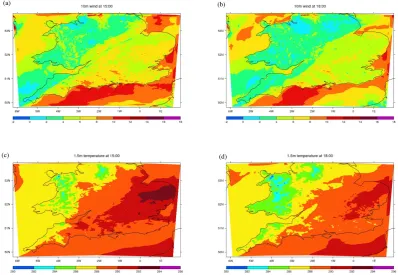
Fig. 6. Control forecast. Left column: 15:00 UTC (T+3), right column: 18:00 UTC (T+6) 20 September 2011. Top row: 10 m wind speed (m s−1), bottom row: 1.5 m temperature (K).
Table 2. Summary of model configurations for the ensemble experiments.
Ensemble name Description IC and LBC perts RP scheme
CTL Control (perturbed ICs and LBCs, no RP scheme) Yes No
IC + BC + RPfix perturbed ICs and LBCs, RP scheme applied once Yes Yes IC + BC + RP30 perturbed ICs and LBCs, RP scheme applied every 30 min Yes Yes IC + BC + RP60 perturbed ICs and LBCs, RP scheme applied every 60 min Yes Yes
RPfix RP scheme applied once No Yes
RP30 RP scheme applied every 30 min No Yes
RP60 RP scheme applied every 60 min No Yes
T+30 min (after the IAU and ILBCU have finished). Experi-ments labelled RP* have no IC and LBC perturbations: their members all use the unperturbed ICs and LBCs of the control member, with model error represented by applying the RP scheme. These ensembles therefore show the effects of using the RP scheme to perturb parameters, without the effects of perturbing the ICs and LBCs.
3 Description of the case and sensitivity tests to inform the modifications to the RP scheme
3.1 Overview
For this study we focus on a case on 20 September 2011 characterised by the passage of a cold front over the
Fig. 7. Sensitivities of the forecasts atT+3 (15:00 UTC) to perturbing parameters to their maximum and minimum values. Top row: difference between perturbed and control forecast at each point, averaged over the domain. Error bars show the standard deviation of the differences. Bottom row: RMS difference between the perturbed and control forecast at each point, averaged over the domain. Left column: 1.5 m temperature. Right column:ucomponent of 10 m wind.
used in ongoing related work (Migliorini, Bannister, Rudd and Baker, in preparation). The second reason for choosing this case is that it has an unusual triple banded structure in the rain band passing over the UK, which was present in the radar rain rate (Fig. 4) but was not captured by the Met Office operational high-resolution deterministic forecast (the UKV forecast; 1.5 km grid length, covering the whole UK; not shown). This triple rain band feature, and the fact that it was not captured by the operational deterministic forecast, makes it an interesting case to study using an ensemble of forecasts. It is not clear from either the model forecasts or the radar observations what the cause of this banded struc-ture is; this is the subject of ongoing work and is beyond the scope of this paper.
We focus on the period 12:00 UTC to 18:00 UTC, and are particularly interested in evaluating the performance and spread of the ensemble at 15:00 UTC (T+3) as this is typ-ically a useful timescale for convective scale forecasts. This should also allow time for model error introduced by the RP scheme to have effect before information coming through the boundaries begins to dominate (Gebhardt et al., 2011).
3.2 Control forecast from the 1.5 km EPS
Fig. 8. Control ensemble rainfall rate (mm h−1) at 15:00 UTC. The control member (member 0) is in the top left-hand corner.
3.3 Parameter sensitivity tests
In order to make the RP scheme suitable to be used in the 1.5 km EPS, we first identified suitable parameters to be per-turbed within the scheme, in addition to those used in the operational scheme. Since work had already been done by Zadra and Lock (2010) to identify extra parameters to be perturbed in the boundary layer scheme after the RP scheme was originally developed, we focus here on parameters in the large-scale precipitation scheme. An extensive set of around 50 parameters known to have some uncertainty was deter-mined by consulting with experts at the Met Office. For each parameter a suitable range of values was chosen such that it was physically sensible while also reflecting the uncertainty in the value of the parameter.
From this extensive list of parameters, a smaller subset was chosen (Table 1). The first nine parameters listed in Table 1 are those used in the operational RP scheme, although some of the ranges have been changed, based on advice by experts. The last seven parameters in Table 1 are those that we have added to the RP scheme. The selection of these parameters was motivated by choosing from the 50 those with the high-est sensitivity, and choosing one parameter for each physical process, in order to minimise the possibility of parameters counteracting each other. Choosing a set of parameters that
collectively control a variety of different processes also has the advantage that the overall effects of the scheme may be less case-dependent. In addition, some parameters were cho-sen to vary together in pairs. These pairs of related parame-ters are indicated in Table 1. Parameparame-tersRicandg0 are re-lated byRic=10/g0; for the other parameter pairs the same random number is used to update their associatedin Eq. (1), which ensures that these pairs of parameters remain corre-lated. In this chosen set of parameters, there are seven pa-rameters from the boundary layer scheme and nine from the large-scale precipitation scheme, but due to the pairings of some parameters there are five independent parameters from the boundary layer scheme and seven independent parame-ters from the large-scale precipitation scheme.
Fig. 9. Spatial distribution of rain rate diagnostics (mm h−1) for the control ensemble. Left column: ensemble mean, middle column: ensem-ble spread and right column: innovation magnitude of the ensemensem-ble mean, at 15:00 UTC (top row) and 18:00 UTC (bottom row) 20 Septem-ber 2011.
imply that perturbing this parameter randomly may introduce a bias.
The sensitivity of the forecast to perturbing each of the pa-rameters to its maximum and minimum value was examined both by computing domain-averaged differences and root-mean-squared (RMS) differences. Difference maps of sur-face variables at different forecast lead times were also ex-amined (not shown). These show that different parameters af-fect the forecast in different parts of the domain. Specifically, the large-scale precipitation parameters have the strongest effects in the region of the rain band, while the effects of boundary layer parameters are generally more widespread, and most strongly affect the north-east part of the domain.
Figure 7 shows the domain-averaged 3 h sensitivities with respect to each of the 12 independent parameters (or param-eter pairs) for 1.5 m temperature and for theucomponent of the 10 m wind. Equivalent plots for 1.5 m RH andv compo-nent of 10 m wind (not shown) show qualitatively similar re-sults to those for 1.5 m temperature and for theucomponent of 10 m wind (respectively), in terms of their relative sensi-tivities to each parameter (although note that the response for 1.5 m RH has the opposite sign to the response for 1.5 m tem-perature, as might be expected). Figure 7a and b show that for all parameters, the domain average effects on the temper-ature and u-component of wind of perturbing a parameter to its maximum value has an opposite sign to perturbing it to its minimum value. However, the bars showing the standard deviation indicate that there is a large variability in the effect of these parameters over the domain. The RMS difference plots (Fig. 7c and d) give a measure of the magnitude of the
sensitivity to each of the parameters. It can be seen that the boundary layer parameter pairs (g0, Ric) and (gmezcla, λmin), and the large-scale precipitation parameter x1r (perturbed only to its maximum value) have the largest effects on both the temperature and u component of wind. The parameter pairs (g0, Ric) and (gmezcla, λmin) affect the wind more, while x1rhas a large impact on the temperature. Although the ef-fects of these parameters dominate in this case, the efef-fects of perturbing the other parameters are not orders of magni-tude smaller. The sensitivity to most of the parameters will be dependent on the atmospheric state (in particular the bound-ary layer stability for the boundbound-ary layer parameters, and the cloud amount and type for the large-scale precipitation pa-rameters), and these results confirm that this is a reasonable set of parameters and ranges to choose in order to simulate model error variability.
4 Evaluation of the control ensemble
In this section we describe the properties of the control en-semble, CTL, which has IC and LBC perturbations but no representation of model error variability.
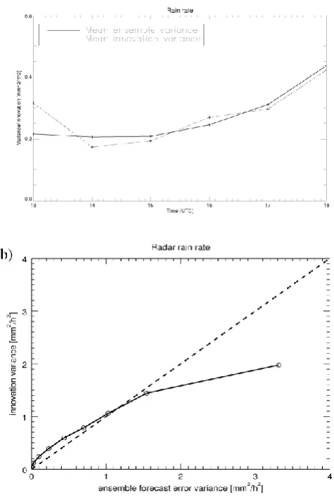
Fig. 10. (a) Domain averaged ensemble variance and innovation
variance for rain rate every hour. (b) Spread-skill plot for the con-trol ensemble. In (b) the data for each grid point for each hour of the forecast are binned into 10 bins by ensemble variance.
this banded structure to form in reality was not well repre-sented in MOGREPS-R. Our hope was that the increased res-olution might lead to some 1.5 km EPS members capturing the second band, but Fig. 8 shows that this ensemble also fails to capture the two bands together in any individual member. Whether this is an inevitable consequence of the lack of mul-tiple bands in the driving model is an open question.
There is generally good agreement in the positioning of the main rain band, although three members (members 1, 13 and 19) have the rain band displaced further to the north. This means that, although the two distinct bands seen in the radar are not captured, these three members do have some rain in roughly the location of the second radar rain band. Several of the ensemble members have more intense rain in the north-east part of the rain band, and in particular some of them have one or two localised regions of heavy rain (e.g. mem-bers 7, 8 and 13) exceeding 16 mm h−1, which is not seen in
Fig. 11. Correspondence ratio for the control ensemble for hourly
rain accumulation.
the radar rain rate. The locations of these localised regions of heavy rain correspond to the two regions of heaviest rain in the ensemble mean at this time (Fig. 9a). By 18:00 UTC the positioning of the rain band in the ensemble mean (Fig. 9d) compares well with the position of the main rain band in the radar (Fig. 5b), although the region of moderately heavy rain off the east coast in the radar is relatively weak in the ensemble mean.
Comparison of the ensemble spread with the innovation magnitude (middle and right columns of Fig. 9) shows that these quantities have quite different spatial distributions at both times shown. In the ensemble spread (Fig. 9b and e) there are more widespread regions of low values of spread, while in the innovation magnitude (Fig. 9c and f) there are more localised regions of higher values. Thus although the domain-averaged quantities (Fig. 10a) appear to be very sim-ilar, this is not due to these quantities having the same spatial distribution. The spread-skill plot produced by binning the data by ensemble variance (Fig. 10b) shows generally good agreement between the ensemble forecast error variance and the innovation variance. For larger ensemble forecast error variances the innovation variance is not as large, which could suggest that the ensemble is overspread in areas with higher rain rates. However, this may be at least partly due to the limited ensemble size (Bowler et al., 2008). These results are qualitatively similar to Fig. 16 in Bowler et al. (2008) and Fig. 15 in Migliorini et al. (2011).
Fig. 12. Probability of rain rate exceeding given thresholds (%) for the control ensemble at 15:00 UTC. Thresholds are (a) 0 mm, (b) 0.2 mm, (c) 1 mm and (d) 2 mm.
are in generally good agreement about the location of the rain band, they disagree in the details of the location of heavier rain. This is supported by Fig. 12 which shows the probabil-ity of rain exceeding given thresholds. For a 0 mm threshold (Fig. 12a), there is a broad region across the domain with 100% probability of rain. In contrast, for higher thresholds (Fig. 12b–d) there are more areas with lower probabilities. For the three thresholds shown in Fig. 12b–d, there is a small region in the centre of the domain with high probabilities. This corresponds to some much smaller regions of rain ex-ceeding 2 mm in the radar (Fig. 5a). In Fig. 12b and c there is some hint of a slightly separated band extending further north than the main rain band, which may be related to the second band seen in the radar (Fig. 5a), although in Fig. 12b and c it does not extend as far north.
The Brier score (BS) for hourly rain accumulation (Fig. 13a) shows an improvement in the skill over time for the 0 and 0.2 mm accumulation thresholds. This improvement over time, particularly after 15:00 UTC, suggests that the in-formation coming through the boundaries at later times im-proves the forecast. There is also a significant improvement with increasing accumulation threshold, which is largely due to the decrease in the number of points exceeding the larger thresholds (Fig. 13b). This increases the number of points that are correctly forecast as not having rain exceeding the threshold, thus effectively improving the BS.
5 Evaluation of the effects of applying the RP scheme
The CTL ensemble represents just one realisation of fore-cast error. Here we examine the ensembles that have model error variability represented using the RP scheme. The fea-tures of each ensemble and the way that each is labelled are described in Sect. 2.5 and in Table 2. Here we show results for one run of each type of ensemble. To confirm that the results presented here are robust and not simply a result of specific combinations of random numbers used in theterm in Eq. (1), these ensemble runs were repeated using differ-ent sets of random numbers. The results from these repeated ensembles were found to be qualitatively similar to those presented here.
Fig. 13. (a) Brier score for the control ensemble for hourly rain
accumulation, calculated using model and radar data resampled to a 13.5 km grid. (b) shows the number of observation data points exceeding each rain accumulation threshold.
5.1 The effects of the RP scheme on ensemble spread
For all the IC + BC + RP* ensembles there is some increase in the ensemble spread compared with the CTL ensem-ble, for the near-surface fields shown in Fig. 14b–d. For hourly rain accumulation (Fig. 14a) there is a slight de-crease in spread in the IC + BC + RP* ensembles compared with the CTL ensemble. Note that the rapid increase in en-semble spread over the first hour of the simulation (until 12:30 UTC) is due to the gradual introduction of the IC per-turbations by the IAU scheme over this period, which means that the ensemble members diverge throughout this time. The RP scheme is first applied at the end of the IAU pe-riod (at 12:30 UTC), causing a divergence in the spread of the four ensembles at this time. For temperature and RH (Fig. 14c and d), the three IC + BC + RP* ensembles have
consistently larger spread than the CTL ensemble. For these variables there is little difference between the three model er-ror ensembles, although IC + BC + RPfix has a slightly larger spread towards the end of the forecast. For 10 m wind speed (Fig. 14b) there is a slight increase in the spread in the IC + BC + RP* ensembles compared with the CTL ensem-ble. The spread for the two ensembles with periodic calls to the RP scheme (IC + BC + RP30 and IC + BC + RP60) has some small jumps at times corresponding to the times that the RP scheme updates the parameters. For hourly rain ac-cumulation (Fig. 14a) the evolution of spread for ensem-bles IC + BC + RP30 and IC + BC + RP60 is less smooth than for ensemble IC + BC + RPfix, and while generally lower than the spread for the CTL ensemble, both ensembles have larger spread between around 16:30 and 17:30 UTC than the IC + BC + RPfix.
The spread gained by applying the RP scheme compared with the CTL ensemble can be compared with the results of Hacker et al. (2011). Their perturbed parameter ensem-ble gave an increase in spread for 2 m temperature of up to 30 % (their Fig. 6a), compared with their control ensem-ble. This compares well with Fig. 14c, which shows an in-crease in spread of 30 % in the last hour or so of the forecast for 1.5 m temperature. Their results also show an increase in spread of around 20 % for 2 m specific humidity (their Fig. 6c), compared with a 15–20 % increase in the spread for RH (Fig. 14d). In contrast to our results, Hacker et al. (2011) show a negligible change in 10 m wind speed, and an increase in spread for precipitation accumulation.
Figure 14a–d show that model error variability alone intro-duces much smaller spread than the IC perturbations, but still a much larger amount than the difference between the spread in the CTL and IC + BC + RP* ensembles. This is consistent with the results of Gebhardt et al. (2011) who found that the effects of their combined physics and LBC perturbations was not the sum of these two perturbations individually. For all four variables shown in Fig. 14a–d the change in spread of the RP* ensembles mirrors the shape of the spread of the IC + BC + RP* ensembles, increasing slightly throughout the forecast. It is interesting to note that the RPfix ensemble still shows an increase in spread throughout the forecast similar to the RP30 and RP60 ensembles, despite the fact that the RP scheme is only applied once. This indicates that the effect of the RP scheme on the spread is due to the members fol-lowing different model manifolds from the first application, and subsequent changes to the manifolds due to repeated ap-plications of the RP scheme in RP30 and RP60 do not in-crease the spread further in a substantial way. The similarity of the spreads between all RP* experiments may also be re-lated to the high autocorrelation coefficient,r, in Eq. (1) and the nonlinear relationships between the parameter values and the forecasts.
Ensemble spread for rainfall accumulation
11:30 12:30 13:30 14:30 15:30 16:30 17:30 18:30 Time
0.0 0.1 0.2 0.3 0.4 0.5
Ensemble spread
Ensemble spread for 10m wind speed
11:30 12:30 13:30 14:30 15:30 16:30 17:30 18:30 Time
0.0 0.2 0.4 0.6 0.8 1.0
Ensemble spread
Ensemble spread for 1.5m temperature
11:30 12:30 13:30 14:30 15:30 16:30 17:30 18:30 Time
0.0 0.2 0.4 0.6
Ensemble spread
Ensemble spread for 1.5m RH
11:30 12:30 13:30 14:30 15:30 16:30 17:30 18:30 Time
0 1 2 3 4
Ensemble spread
(c)
(a) (b)
(d)
Fig. 14. Evolution of ensemble spread with forecast time for the different ensembles, for (a) hourly rainfall accumulation (mm), (b) 10 m
wind speed (m s−1), (c) 1.5 m temperature (K) and (d) 1.5 m RH (%).
between members in the location of the rain band. This is in agreement with plots of the probability of rain exceed-ing 0 mm for the IC + BC + RP* ensembles (equivalent to Fig. 12a) (not shown) which show broader regions with 100 % probability of rain than for the CTL ensemble. For higher thresholds (Fig. 15b–d) there is no significant change in the CR for the IC + BC + RP* ensembles compared with the CTL ensemble. The RP* ensembles have higher CR val-ues than the CTL and IC + BC + RP* ensembles throughout the forecast for all thresholds (Fig. 15a–d). This is consistent with the much lower spread seen in rain accumulation for the RP* ensembles (Fig. 14a). The RP60 ensemble has con-sistently lower CR values than the other RP* ensembles for all thresholds, indicating more variability between ensemble members in this case. This is in agreement with Fig. 14a which shows a slightly higher spread for the RP60 ensem-ble than for RP30 and RPfix.
Figure 16a shows that the ensemble mean for the IC + BC + RPfix ensemble has a larger peak and a slightly narrower rain band than the ensemble mean for the CTL ensemble (Fig. 9a). The ensemble spread for the IC + BC + RPfix ensemble extends over a narrower band than the CTL ensemble (Fig. 16b compared with Fig. 9b), which is consistent with the reduction in domain-averaged spread seen in Fig. 14a. The innovation magnitude for the IC + BC + RPfix ensemble (Fig. 16c) is very similar to the in-novation magnitude for the CTL ensemble (Fig. 9c), and sim-ilarly for the IC + BC + RP30 and IC + BC + RP60 ensembles
(not shown). Therefore the addition of model error has not improved the relationship between the spatial distributions of ensemble spread and innovation magnitude.
5.2 The effects of the RP scheme on the forecast skill
The skill of each ensemble forecast was evaluated using the CRPS, as shown in Fig. 17 (accounting for observation error as described in Sect. 2.4). The observation error variance for each quantity was estimated from spread-skill plots for this case as the value of the skill for zero spread. The values used are specified in the figure caption. Repeating the calculations, but with zero observation error gives qualitatively similar re-sults, which suggests that the results are not sensitive to the exact observation error variance values used.
CR for 0.2mm rain accumulation
13 14 15 16 17 18
Time 0.0
0.2 0.4 0.6 0.8 1.0
CR
CR for 1mm rain accumulation
13 14 15 16 17 18
Time 0.0
0.2 0.4 0.6 0.8 1.0
CR
CR for 2mm rain accumulation
13 14 15 16 17 18
Time 0.0
0.2 0.4 0.6 0.8 1.0
CR
CR for 0mm rain accumulation
13 14 15 16 17 18
Time 0.0
0.2 0.4 0.6 0.8 1.0
CR
(c) (d)
(a) (b)
Fig. 15. Correspondence ratio for hourly rain accumulation for all the ensembles. Thresholds are (a) 0 mm, (b) 0.2 mm, (c) 1 mm and (d)
2 mm.
Both investigations, however (results not shown), showed no systematic signals to suggest that the LBC information is re-sponsible for the decrease of CRPS (although this may be due to an insufficient observational sample at any given lead time and so this remains an open question). The improve-ment in skill with lead time for temperature and winds may be due to the effect of the readjustment of the forecast en-semble to a more balanced set of states after the effect of the inflation on the initial ensemble spread. As discussed in Sect. 2.1, the inflation is a spatially constant factor – deter-mined from temperature and winds power spectra at selected levels – imposed on the ICs as determined by the ETKF. Ar-guably, a sub-optimal inflation on the initial ensemble spread could cause spurious gravity waves leading to loss of skill in the first hour into the forecast and subsequent improvements in skill would be achieved when the effects of the initial in-flation are “forgotten” by the forecast ensemble.
The IC + BC + RP* ensembles have consistently better skill than the CTL ensemble, with a significant improvement in skill at and after the 4 h lead time. For 1.5 m RH (Fig. 17d) the skill for all ensembles gets worse over the first two hours, followed by an improvement from the 3 h lead time. As with 1.5 m temperature, the IC + BC + RP* ensembles show con-sistently better skill than the CTL ensemble, with the dif-ferences becoming more significant after the 2 h lead time. For surfaceuandv wind (Fig. 17e and f) there is large un-certainty in these results, shown by the standard error bars. There is no significant difference in the CRPS between
en-sembles, indicating that the RP scheme has little impact on the skill of the wind forecast. For rain rate and hourly rain ac-cumulation (Fig. 17a and b) all ensembles show an improve-ment in skill between the 1 and 2 h lead times, followed by a degradation in skill over the remainder of the forecast. For the first 2 h, the IC + BC + RP* ensembles show an improve-ment in the skill compared with the CTL ensemble, which is particularly significant in the rain accumulation at the 1 h lead time. After this the IC + BC + RP* ensembles have a sig-nificantly worse skill than the CTL ensemble. These results are consistent with results using the PSS (Fig. 18). In the first 2 h of the forecast the PSS is positive for all thresholds, show-ing that the IC + BC + RP* ensembles perform slightly better than the CTL ensemble; after this time the PSS is negative, showing that the IC + BC + RP* ensembles are less skillful than the CTL ensemble according to this diagnostic. For the higher thresholds (Fig. 18c and d) the PSS is approximately zero at 15:00 UTC, indicating no change in the skill at this time for these thresholds. All three IC + BC + RP* ensembles show similar PSS values throughout much of the forecast, although for the 0 mm threshold (Fig. 18a) IC + BC + RPfix performs worse than the other ensembles towards the end of the forecast.
Fig. 16. Rain rate diagnostics for the IC + BC + RPfix ensemble (mm h−1). (a) ensemble mean, (b) ensemble spread and (c) innovation magnitude of the ensemble mean, all at 15:00 UTC 20 September 2011.
perturbed ICs and LBCs. This is likely due to the smaller spread in the RP* ensembles compared with the others.
For all ensembles shown in Fig. 17 (i.e. with and with-out model error variability) and for the near-surface quanti-ties (1.5 m temperature and RH and 10 m wind) the forecasts show a tendency to improve throughout the forecast. This is indicated by a decrease of the CRPS with time. This may be due to the spin-up of the model after the IAU has finished and to large-scale information coming in from the boundaries. All ensembles show an improvement in rainfall skill for the first 2 h of the forecast, with the IC + BC + RP* ensembles performing better in this period. In contrast, all ensembles show a worsening of skill in rainfall towards the end of the forecast, and the IC + BC + RP* ensembles show worse skill than the CTL ensemble for rain rate and accumulation. This may be due to inconsistencies between fields in the interior of the domain (for which some parameters have been perturbed) and the LBCs (which have not been perturbed). However, the validity of this idea is difficult to demonstrate with just one case study.
6 Conclusions
In this paper we have evaluated the effects of using the ran-dom parameters (RP) scheme as a method of representing model error in the 1.5 km EPS for a case on 20 Septem-ber 2011 in which a frontal rain band crossed through the domain. Although it is difficult to draw conclusions from one case study only, we have shown that the RP scheme in this convective-scale EPS can actually reduce the ensemble vari-ability for some variables.
6.1 Summary of results
The standard RP scheme (used operationally in MOGREPS) was used as a basis for the representation of model error un-certainty, and modifications were made to make it suitable for use in the convective-scale 1.5 km EPS. A set of extra param-eters to be perturbed were identified in the large-scale precip-itation scheme, in addition to the existing boundary layer and large-scale precipitation parameters (Table 1). Some pairs of related parameters were varied together (using the same
ran-dom number), with the intention of controlling each physical process by only one parameter or one pair of parameters. Pa-rameter sensitivity testing on forecasts showed that there was some sensitivity to all the chosen parameters when perturbed individually, and none of the perturbed forecasts gave physi-cally unrealistic results.
Seven ensembles were run with different configurations: the control ensemble had IC and BC perturbations only; three ensembles had IC and BC perturbations and model error rep-resented by the RP scheme, with parameter values updated with different periods; and three ensembles had no IC or BC perturbations but did have model error represented by the RP scheme, with the same three update periods.
The control ensemble was found to represent the main rain band reasonably well, but all members failed to capture the two separate rain bands seen in the radar in the model’s do-main. The position of the main rain band, however, in this ensemble was positioned in some members at locations oc-cupied by the second rain band in the radar. This was also the case for the ensembles with model error.
Fig. 17. CRPS for (a) rain rate, (b) hourly rain accumulation, (c) 1.5 m temperature, (d) 1.5 m RH, (e)ucomponent of 10 m wind and (f)v component of 10 m wind. The CRPS shown is the mean CRPS over the domain for each ensemble; error bars show the standard error in the mean. The observation error standard deviations used in the calculation are (a)σo=0.47mm h−1, (b)σo=0.47mm, (c)σo=0.69K, (d) σo=4.72 %, (e)σo=1.54m s−1and (f)σo=1.54m s−1. These values were estimated from spread-skill plots for this case.
1.5 m relative humidity, as compared with the control ensem-ble. For rainfall, there was an improvement in skill at the start of the forecast for the IC + BC + RP* ensembles compared with the control, but a reduced skill in the last few hours. This may be due to inconsistencies between the interior and the boundaries of the domain, which may lead to incorrect rainfall amounts later in the forecast.
The results for both the spread and the skill indicate that perturbing the parameters periodically throughout the fore-cast has little impact on the forefore-cast spread or skill com-pared with perturbing the parameters once and holding them
fixed for the rest of the forecast. However, perturbing the pa-rameters only once means that less of the parameter space will be spanned.
PSS for 0mm rain accumulation
13 14 15 16 17 18
Time (UTC) -0.6
-0.4 -0.2 -0.0 0.2 0.4 0.6
precip skill score
PSS for 1mm rain accumulation
13 14 15 16 17 18
Time (UTC) -0.6
-0.4 -0.2 -0.0 0.2 0.4 0.6
precip skill score
PSS for 0.2mm rain accumulation
13 14 15 16 17 18
Time (UTC) -0.6
-0.4 -0.2 -0.0 0.2 0.4 0.6
precip skill score
PSS for 2mm rain accumulation
13 14 15 16 17 18
Time (UTC) -0.6
-0.4 -0.2 -0.0 0.2 0.4 0.6
precip skill score
(a) (b)
(c) (d)
Fig. 18. PSS for hourly rain accumulation for the IC + BC + RP* ensembles with reference to the CTL ensemble for (a) 0 mm, (b) 0.2 mm, (c) 1 mm and (d) 2 mm thresholds.
6.2 Further work
An obvious limitation of this study is that we have considered only one particular case. This was due to time constraints and upgrades to the modelling system which meant that it was not possible to run further cases with the same model setup. Re-peating these experiments with different cases, in particular for different synoptic situations such as convective showers rather than a synoptically forced frontal system would give a broader picture of the usefulness of the RP scheme. We ex-pect that for different synoptic situations there would be dif-ferences in the relative sensitivity to each of the parameters. For example, we expect that in a convective case the pertur-bations made to the large-scale precipitation parameters may have a larger effect than in the case discussed here.
A further limitation is our constraint to using the existing formulation of the RP scheme as a basis for our study. One potential issue with this setup is that each time the parame-ters are perturbed the model is “kicked” into a different state corresponding to a particular set of parameter values. While the formulation of the autoregression Eq. (1) used in the RP scheme ensures that the parameters remain within a certain range of their previous values, this did still introduce some jumpiness in the wind and rain fields, which is not desirable. An alternative approach would be to update the parameter values more frequently (e.g. every time step, which we might call RPts), but change the autoregression constantrin Eq. (1) to be closer to unity, and/or reduce the range of the shock.
This would allow a smooth evolution of parameters. By ex-trapolating the results in this study, we hypothesize that this smoother approach would give a more skillful forecast than the method used here, but may not give any additional in-crease in ensemble spread. It would also require tuning ofr
and, which would be a time-consuming process.
The possible ways in which the RP scheme may be applied raises some interesting issues. At one end of the scale RPfix allowsnsets of parameters (wherenis the number of ensem-ble members) to be applied in forecasts that each follow pre-cisely the model equations. At the other end of the scale RPts allows more of parameter space to be explored, but no mem-ber will follow the same model equations. Strictly speaking this will lead to loss of continuity (of e.g. mass, water, energy, etc.), but this may actually be a desirable feature given that the model equations are imperfect and the conserved quanti-ties are imperfectly known anyway. Each strategy represents a different philosophical approach to representing model er-ror variability with variable parameters and a comparison would make an interesting piece of future work.
it could be useful for nowcasting and very short forecasts. A potential application of the RP scheme could be to use it within an hourly cycling system as an alternative to the in-flation factor as a method of increasing the ensemble spread. It would also be of use on a larger domain, such as that of the new MOGREPS-UK ensemble, which covers the whole of the UK, and therefore the interior of the domain would be less strongly influenced by the LBCs.
Ongoing work aims to investigate the effects of the RP scheme on forecast error covariance statistics and covari-ance length scales (Migliorini, Bannister, Rudd and Baker, in preparation) and on the inherent balances that are obeyed by the ensemble (Bannister, Migliorini, Baker and Rudd, in preparation). These have applications to informing the appro-priate formulation of the background error covariance matrix used in convective-scale data assimilation systems.
Acknowledgements. This work was funded by the Natural
Envi-ronment Research Council (NERC) under the DIAMET project (Grant ref. NE/I005234/1).The authors wish to thank Ian Boutle and Jonathan Wilkinson for their advice on parameterisation schemes; Emilie Carter, Jean-Francois Caron, Giovanni Leoncini, David Simonin, Simon Wilson and Roger Brugge for technical help; and Sue Ballard, Neill Bowler and Jonathan Flowerdew for helpful discussions on this work. We are also grateful for constructive comments from two anonymous referees and editors of NPG (Roberto Buizza and Olivier Talagrand), which helped to improve the paper. We thank NERC and the Met Office for use of the MetUM and the MONSooN supercomputing facility.
Edited by: R. Buizza
Reviewed by: two anonymous referees
References
Berner, J., Shutts, G. J., Leutbecher, M., and Palmer, T. N.: A spec-tral stochastic kinetic energy backscatter scheme and its impact on flow-dependent predictability in the ECMWF Ensemble Pre-diction System, J. Atmos. Sci., 66, 603–629, 2009.
Berner, J., Ha, S.-Y., Hacker, J. P., Fournier, A., and Snyder, C.: Model uncertainty in a mesoscale ensemble prediction system: Stochastic versus multiphysics representations, Mon. Weather Rev., 139, 1972–1995, 2011.
Bishop, C. H., Etherton, B. J., and Majumdar, S. J.: Adaptive sam-pling with the ensemble tranform Kalman filter. Part I: Theoreti-cal aspects., Mon. Weather Rev., 129, 420–436, 2001.
Bouttier, F., Vié, B., Nuissier, O., and Raynaud, L.: Impact of Stochastic Physics in a convection-permitting ensemble, Mon. Weather Rev., 140, 3706–3721, 2012.
Bowler, N. E., Arribas, A., Mylne, K. R., Robertson, K. B., and Beare, S. E.: The MOGREPS short-range ensemble prediction system, Q. J. Roy. Meteorol. Soc., 134, 703–722, 2008. Bright, D. R. and Mullen, S. L.: Short-range ensemble forecasts of
precipitation during the Southwest Monsoon, Weather Forecast., 17, 1080–1100, 2002.
Buizza, R., Miller, M., and Palmer, T. N.: Stochastic representation of model uncertainties in the ECMWF Ensemble Prediction Sys-tem, Q. J. Roy. Meteorol. Soc., 125, 2887–2908, 1999.
Caron, J.-F.: Mismatching perturbations at the lateral boundaries in limited-area ensemble forecasting: A case study, Mon. Weather Rev., 141, 356–374, 2013.
Clark, A. J., Gallus Jr., W. A., Xue, M., and Kong, F.: Growth of spread in convection-allowing and convection-parameterizing ensembles, Weather Forecast., 25, 594–612, 2010.
Clark, A. J., Kain, J. S., Stensrud, D. J., Xue, M., Kong, F., Coniglio, M. C., Thomas, K. W., Wang, Y., Brewster, K., Gao, J., Wang, X., Weiss, S. J., and Du, J.: Probabilistic precipitation forecast skill as a function of ensemble size and spatial scale in a convection-allowing ensemble, Mon. Weather Rev., 139, 1410–1418, 2011. Davies, T., Cullen, M. J. P., Malcolm, A. J., Mawson, M. H.,
Stan-iforth, A., White, A. A., and Wood, N.: A new dynamical core for the Met Office’s global and regional modelling of the atmo-sphere, Q. J. Roy. Meteorol. Soc., 131, 1759–1782, 2005. Fresnay, S., Hally, A., Garnaud, C., Richard, E., and Lambert,
D.: Heavy precipitation events in the Mediterranean: sensitiv-ity to cloud physics parameterisation uncertainties, Nat. Hazards Earth Syst. Sci., 12, 2671–2688, doi:10.5194/nhess-12-2671-2012, 2012.
Gebhardt, C., Theis, S. E., Paulat, M., and Bouallègue, Z. B.: Un-certainties in COSMO-DE precipitation forecasts introduced by model perturbations and variation of lateral boundaries, Atmos. Res., 100, 168–177, 2011.
Gregory, D. and Rowntree, P. R.: A mass flux convection scheme with representation of cloud ensemble characteristics and stability-dependent closure, Mon. Weather Rev., 118, 1483– 1506, 1990.
Hacker, J. P., Snyder, C., Ha, S.-Y., and Pocernich, M.: Linear and non-linear response to parameter variations in a mesoscale model, Tellus, 63A, 429–444, 2011.
Hersbach, H.: Decomposition of the Continuous ranked probabil-ity score for ensemble prediction systems, Weather Forecast., 15, 559–570, 2000.
Lean, H. W., Clark, P. A., Dixon, M., Roberts, N. M., Fitch, A., Forbes, R., and Halliwell, C.: The Met Office global three-dimensional variational data assimilation scheme, Q. J. R. Me-teorol. Soc., 131, 1759–1782, 2008.
Lin, J. W.-B. and Neelin, J. D.: Influence of a stochastic moist convective parameterization on tropical climate variability, Geo-phys. Res. Lett., 27, 3691–3694, 2000.
Lock, A. P., Brown, A. R., Bush, M. R., Martin, G. M., and Smith, R. N. B.: A new boundary layer mixing scheme. Part I: scheme description and single-column model tests, Mon. Weather Rev., 128, 3187–3199, 2000.
Migliorini, S., Dixon, M., Bannister, R., and Ballard, S.: Ensemble prediction for nowcasting with a convection-permitting model – I: description of the system and the impact of radar-derived sur-face precipitation rates, Tellus, 63, 468–496, doi:10.1111/j.1600-0870.2010.00503.x, 2011.
Shutts, G.: A kinetic energy backscatter algorithm for use in ensem-ble prediction systems, Q. J. Roy. Meteorol. Soc., 131, 3079– 3102, 2005.
Stainforth, D. A., Aina, T., Christensen, C., Collins, M., Faull, N., Frame, D. J., Kettleborough, J. A., Knight, S., Martin, A., Murphy, J. M., Pianl, C., Sexton, D., Smith, L. A., Spicer, R. A., Thorpe, A. J., and Allen, M. R.: Uncertainty in predictions of the climate response to rising levels of greenhouse gases, Nature, 433, 403–406, 2005.
Stensrud, D. J., Bao, J.-W., and Warner, T. T.: Using initial condition and model physics perturbations in short-range ensemble simula-tions of mesoscale convective systems, Mon. Weather Rev., 128, 2077–2107, 2000.
Vié, B., Molinié, G., Nuissier, O., Vincendon, B., Ducrocq, V., Bouttier, F., and Richard, E.: Hydro-meteorological evaluation of a convection-permitting ensemble prediction system for Mediter-ranean heavy precipitating events, Nat. Hazards Earth Syst. Sci., 12, 2631–2645, doi:10.5194/nhess-12-2631-2012, 2012.
Webster, S., Brown, A. R., Cameron, D. R., and Jones, C. P.: Im-provements to the representation of orography in the Met Office Unified Model, Q. J. Roy. Meteorol. Soc., 129, 1989–2010, 2003. Wilks, D. S.: Statistical methods in the atmospheric sciences,
Else-vier Academic Press, 2nd Edn., 2006.
Wilson, D. R. and Ballard, S. P.: A microphysically based precipi-tation scheme for the Meteorological Office Unified Model, Q. J. Roy. Meteorol. Soc., 125, 1607–1636, 1999.