www.nonlin-processes-geophys.net/16/607/2009/ © Author(s) 2009. This work is distributed under the Creative Commons Attribution 3.0 License.
Nonlinear Processes
in Geophysics
The stochastic multiplicative cascade structure of deterministic
numerical models of the atmosphere
J. Stolle1, S. Lovejoy1, and D. Schertzer2,3
1Physics, McGill University, 3600 University St., Montreal, Que. H3A 2T8, Canada 2CEREVE, Universit´e Paris Est, Marne-la-Vall´ee, France
3M´et´eo France, 1 Quai Branly, Paris 75005, France
Received: 16 February 2009 – Revised: 1 July 2009 – Accepted: 22 August 2009 – Published: 26 October 2009
Abstract. By direct statistical analysis we show that over
almost all their range of scales and to within typically bet-ter than±1%, atmospheric fields obtained from analyses and numerical integrations of atmospheric models have the mul-tifractal structure predicted by multiplicative cascade mod-els. We quantify this for the horizontal wind, tempera-ture, and humidity fields at 5 different pressure levels for the ERA40 reanalysis, the Canadian Meteorological Centre Global Environmental Multiscale (CMC, GEM) model, as well as the National Oceanographic and Atmospheric Ad-ministration Global Forecasting System (NOAA, GFS). We investigate the additional prediction that the cascade belongs to a universal multifractal basin of attraction. By demonstrat-ing a “Levy collapse” of the statistical moments to within±2 to±5% over most of the range of scales, we conclude that there is good evidence for this. Finally, we discuss how this stochastic multiplicative cascade structure can be exploited in improving ensemble forecasts.
1 Introduction
1.1 Numerical weather prediction and cascades
Richardson’s seminal book “Weather prediction by numeri-cal process” (1922) is venerated as the pioneering work in numerical atmospheric modelling. With a lapse of about 30 years, Richardson’s idea was taken up by generations of atmospheric scientists; the result is modern ensemble fore-casting systems. However in the same book, and in a subse-quent papers (especially Richardson, 1926), the seed of an-other idea was sown: that atmospheric dynamics might re-peat scale by scale in a cascade-like manner. In other words
Correspondence to: J. Stolle
Richardson suspected that – if viewed correctly – the seem-ing complexity of the brute force numerics might hide scale by scale simplicity.
In the case of cascades, he was about 40 years ahead of his time: it was not until the 1960’s, that explicit multiplicative cascade models were first developed (Novikov and Stewart, 1964; Yaglom, 1966; Mandelbrot, 1974). These models are based on the scale symmetry (broken only by viscosity at small scales and the forcing at large scales), by scale conser-vation of energy flux and the Fourier localness of the non-linear interactions (so that structures of a given scale mostly interact with other structures of similar scale). These mul-tiplicative cascades can be understood as attempts to deduce the implications of some (but not all) of the symmetries of the governing equations. Since the mid 1980’s it was realized that multiplicative cascade processes are very general; they are the generic multifractal process. Today, their nontrivial statistical properties are relatively well understood and they have been applied throughout physics and the geosciences.
1.2 Cascades in geophysical turbulence
“reanalyses” that it uses are earlier and slightly lower resolu-tion versions of some of the data analysed here. The authors came to some strong conclusions: that there was no evidence fork−5/3ork−3behaviours nor for any upscale transient en-ergy transfer (the usual signature of 2-D turbulence).
Whereas the great majority of turbulence theories are isotropic – or at least quasi isotropic (they have the same ex-ponents but not necessarily the same prefactors in all direc-tions) – empirical studies of the vertical atmospheric struc-ture, e.g., Van Zandt (1982), Schertzer and Lovejoy (1985), Dewan and Good (1986), Gardner (1994), Dewan (1997), Lilley et al. (2004), Lilley et al. (2008), show on the con-trary that the turbulence is anisotropic, with vertical expo-nents different from those in the horizontal so that the strat-ification is scaling. They therefore require anisotropic theo-ries such as the quasi-linear gravity wave theotheo-ries – e.g. the Saturated Cascade Theory (Dewan and Good, 1986; Dewan, 1997) or the Diffusive Filtering Theory (Gardner, 1994) -or the strongly nonlinear 23/9D buoyancy flux/energy flux model (Schertzer and Lovejoy, 1985).
Recent analyses of massive quantities of global scale satel-lite data (visible, infra-red, passive and active microwave wavelengths) have provided new impetus for attempting to test multiplicative cascades on atmospheric models. These studies show empirically that to within≈±1%, the energy containing short and long wave atmospheric radiances re-spect the predictions of multiplicative cascades from plane-tary scales down to at least several kilometres (Lovejoy et al., 2001, 2009a) so that the relevant sources and sinks of fluxes are likely to be scaling. Similarly, Lovejoy et al. (2009c, d) showed that the vertical structure of horizontal wind, pas-sive scalars, temperature, pressure, humidity, potential tem-perature, etc. also have cascade structures down to<≈5 m with outer scales in the range 1–30 km (depending on the field). The picture that emerges from this wide range and anisotropic cascade structure is at odds with the standard model of atmospheric dynamics which involves a “dimen-sional transition” between isotropic 3-D and isotropic 2-D turbulence (the “meso-scale gap”). Indeed, a recent survey (and criticism) of empirical studies over the last 30 years (Lilley et al., 2004, 2008; Lovejoy et al., 2008) shows that the classical studies of Gage and Nastrom (1986) (the GASP experiment) and Cho and Lindborg (2001) (MOZAIC) must be reconsidered, especially their conclusions about spectral breaks and the 2-D turbulence nature of the large scales. The key to this re-evaluation is partly the use of much higher qual-ity modern data (especially from lidar and drop sondes), but also the demonstration that in anisotropic (but scaling) turbu-lence that the nature of aircraft trajectories – whether on iso-machs, isobars, or isoheights), as well as the effect of their vertical fluctuations must be more carefully taken into ac-count. For example, vertical fluctuations of the aircraft may themselves lead to spurious scale breaks and spurious expo-nents (the stratosphere; Lovejoy et al., 2004). Alternatively, the exponents obtained from aircraft flying along isobars –
as they invariably do in the troposphere for air traffic control reasons – can yield exponents spuriously close to the vertical (rather than horizontal) values; they yield spectra exponents of≈−2.4 (rather than≈−5/3) at large scales (Lovejoy et al., 2009c). It is interesting to note that the models discussed here are all hydrostatic so that the “horizontal” levels we an-alyze are actually isobars rather than isoheights. The fact that the wind spectra along isobars and isoheights are quite differ-ent (k−2.4rather thank−5/3)is important and helps explain the model statistics – which for the wind is also close tok−2.4
on isobars; this will be discussed elsewhere.
If the velocity field has a scaling cascade structure, then we expect that there is also a temporal cascade structure so that the cascades are actually in space-time. We confirm this in a forthcoming publication, where we discuss the relationship between the spatial and temporal structures (Stolle, 2009; Stolle et al., 2009). Lovejoy and Schertzer (2009) gives a recent review of some of this work showing the ubiquity of space-time cascade structures and arguing that it allows for a new synthesis of nonlinear dynamics with state of the art atmospheric data. To summarize: it now seems that for the models to be realistic, they must have cascade structures, too.
1.3 Cascades in direct numerical simulations
Before turning our attention to the analysis of atmospheric models, we should also mention the related field of pure hy-drodynamic turbulence which is often considered more fun-damental than atmospheric turbulence, but where the same issues have arisen. They too can involve structures span-ning huge ranges of scale and despite intense efforts over more than 50 years, analytic approaches have been largely ineffective; given their successes elsewhere in fundamental physics, this is perhaps surprising. The limitations of statis-tical closure, renormalization, and other kindred analystatis-tical techniques have lead to the development of two main alter-natives: brute force numerics and phenomenological models, especially cascades.
Although Direct Numerical Simulations (DNS; i.e. with-out subgrid “parameterizations”) of Navier Stokes (NS) equations have been made since Orszag and Patter-son (1972), it was not until Vincent and Meneguzzi (1991) that computers were powerful enough to allow for simula-tions large enough to display hints of the Kolmogorovk−5/3
1.4 Goals and structure
The aim of this paper is thus to test the predictions of multi-plicative cascades on the spatial structure of various numer-ical models of the atmosphere. This paper is structured as follows. In Sect. 2 we review the basic theory including the predictions of the multiplicative models and different meth-ods of estimating fluxes. In Sect. 3 we describe the data sets and present the basic results and in Sect. 4 we conclude.
2 Multiplicative cascade models
2.1 Basic statistics
During the 1960’s and early 1970’s, intermittency was in-creasingly acknowledged as an important phenomenon, but its effect was usually considered small, associated primar-ily with small corrections to the spectral exponents. The main statistical models (such as those used in statistical clo-sures) assumed “quasi-Gaussian statistics”. In order to ob-tain a Gaussian model with the classical Kolmogorov law
1v=ε1/31x1/3(for velocity fluctuations1v over distances
1x)– the real space equivalent of what is given in Fourier space in Kolmogorov (1941) –, it is sufficient to take the en-ergy fluxεas a Gaussian white noise process and giveε1/3
a (fractional) integration of order 1/3 (i.e., a power law fil-ter of order−1/3): the resultingvis a “fractional Brownian motion”.
In order to take into account intermittency, it suffices to replace the Gaussianε in the above model by the result of a multiplicative cascade; this is the Fractionally Integrated Flux model (Schertzer and Lovejoy, 1987). In multiplicative cascades, large structures are broken up into smaller daugh-ter structures which multiplicatively modulate the flux; this process is repeated to smaller and smaller scales. Normal-ized cascade processes generally lead to multifractal fields with statistics:
ϕλq
=λK(q);λ=L/ l (1a)
where “<.>” indicates ensemble (statistical) averaging,ϕis the turbulent flux normalized such that<ϕλ>=1,K(q)is a convex function describing the scaling behaviour of theqt h
moment,λis the ratio of the (large) scaleL, where the cas-cade starts, to the scale of observationl(see Monin and Ya-glom (1975) for an early discussion of cascades or Schertzer and Lovejoy (1987) for the “codimension multifractal for-malism” used throughout this paper). In comparison, the quasi-Gaussian (nonintermittent) classical model is the (triv-ial) special caseK(q)=0.
The usual “discrete in scale” model reproducing Eq. (1) is to consider a uniform (constant) large scale fluxϕ0(=1) which is iteratively divided into random substructures with the scale being reduced by integer ratios λ0 at each step (usuallyλ0=2). These smaller substructures multiplicatively
modulate the larger scale field by independent identically dis-tributed “multiplicative incrementsδϕ” so that afternsteps, at a given location in the space, the field ϕn is given by
ϕn=ϕ0 n
Q
i=1
δϕi while the overall scale range is λ=λno. If hδϕqi = λK(q)
0 we easily see that
ϕnq = λK(q). Since the cascade is multiplicative, its logarithm0n=logεn, the “gen-erator” is additive: 0n=00+
n
P
i
10i (with10i=log(δεi)). It is therefore not surprising that – due to the additive central limit theorem for the sums of identical independently dis-tributed random variables – there exist specific (stable, at-tractive) “universal” forms for the exponentK(q):
K(q)= C1
(α−1)(q
α−q), (1b)
where 0≤C1≤d is the “codimension of the mean”, which characterizes the sparseness of the set that gives the dominant contribution to the first order statistical moment (the mean),
dis the dimension of the space over which the cascade is ob-served (Schertzer and Lovejoy, 1987). The expression “dom-inant contribution” is an asymptotic result valid for largeλ. In this limit there is an exact one to one correspondence be-tween singularities (γ ) and statistical moments (Parisi and Frisch, 1985): γ=K’(q)so that the singularity correspond-ing to q=1 is K’(1)=C1. In addition, the same arguments show that the codimension (the difference of the dimension of spacedand the fractal dimension of this singularity) also equalsC1. The multifractal index 0≤α≤2 characterizes the degree of multifractality, i.e. the shape of the K(q) func-tion. It is also the Levy index of the generator. If the cascade is uni/mono- fractal, then α=0, whereas α=2 corresponds to the “lognormal” multifractal. A “universal multifractal” is the basin of attraction for wide variety of different multiplica-tive processes. Forα<2, Eq. (1b) is only valid forq≥0; the reason is thatεis the exponential of an extremal Levy vari-able and whenα<2, the latter has diverging moments for all
q<0. This means that the probability density ofεhas a
loga-rithmic singularity for smallε(except forα=2, the Gaussian case).
In our analyses, we will see that the universal form (Eq. 1b) fits the empiricalK(q)quite well so that irrespective of whether the numerical models are indeed universal multi-fractals, the parametersC1,αgive very convenient parame-terizations for their forms. Indeed, we have already seen that
As we have seen from the brief history above, the hy-pothesis that high Reynolds number turbulence respects mul-tiplicative cascades is physically based, so the paper aims to test the hypothesis on numerical simulations. While it might be possible that non-multiplicative processes may ex-ist which satisfy Eq. (1a) (and perhaps even Eq. 1b); to our knowledge no such alternative models have been proposed.
2.2 Estimating the turbulent fluxes
In order to test Eq. (1a), we must therefore use an approach that does not require a priori assumptions about the physi-cal nature of the relevant fluxes nor of their sphysi-cale symmetries (isotropic or otherwise). If atmospheric dynamics are con-trolled by scale invariant turbulent cascades of various (scale by scale) conserved fluxesϕ, then in a scaling regime, the fluctuations1f (1x)in an observablef (e.g. wind, temper-ature or radiance) over a distance1xare related to the turbu-lent fluxes by a relation of the form1f (1x)=ϕ1xH. This relation is a generalization of the classical laws of turbulence. For example, the Kolmogorov (1941) law for velocity fluc-tuations hasH=1/3 andϕ=εη,η=1/3 (εis the energy flux), whereas the Corrsin-Obukhov law of passive scalar advec-tion hasϕ=χ1/2ε−1/6whereχis the passive scalar variance flux (Corrsin, 1951 and Obukhov, 1949). Without knowing
ηorH – nor even the physical nature of the flux – we can use this to estimate the normalized (nondimensional) fluxϕ’ at the smallest resolution of our data:
ϕ0=ϕ/hϕi =1f/h1fi. (2)
Note that if the fluxes are realizations of pure multiplica-tive cascades then the normalizedηpower fluxes, εη/hεηi, are also pure multiplicative cascades, so that ϕ0=εη/hεηi is a normalized cascade quantity. The fluctuation 1f (l), at small scales 1x=l can be estimated in various ways; in 1-D a convenient method is to use absolute first differ-ences: 1f (l)= |f (x+l)−f (x)| or absolute second dif-ferences: 1f (l)= |(f (x+l)+f (x−l)) /2−f (x)|. These “poor man’s wavelets” are usually adequate – when as is typically the case 0≤H≤1 or 0≤H≤2 (first or second or-der differences, respectively) – but alternatively other def-initions of fluctuations (other wavelets) could be used. In 2-D, convenient definitions of fluctuations (used below) are the (finite difference) Laplacian (estimated as the difference between the value at a grid point and the average of its neigh-bours:1f3=|f (x, y)−(f (x+l, y)+f (x−l, y)+f (x, y+l)
+f (x, y−l))/4|),or the modulus of a finite difference
es-timate of the gradient vector. The resulting high resolution flux estimates can then be degraded (by averaging) to lower resolutions.
Since empirical data are nearly always sampled at scales much larger than the dissipation scales, the above scaling range based technique has wide applicability. In numerical models however, where we have data down to the (model) dissipation range, we find that the approach still works but
that the interpretation is a little different. To see this, con-sider the example of the energy fluxε, recalling that at the dissipation scale:
ε≈νv· ∇2v (3)
whereνis the viscosity,vthe velocity (this is obtained from the Navier-Stokes equation by takingε=∂v2/∂t and ignor-ing the dynamic terms which are unimportant for dissipa-tion). Standard manipulations (e.g. Landau and Lifshitz, 1963) give:
ε≈ν
3
X
i=1 3
X
j=1
∂v
i
∂xj +∂vj
∂xi
2
≈ν
1v
1x
2
(4)
so that if1xis in the dissipation range (e.g. the finest reso-lution of the model) then:
1v≈ε
ν
1/2
1x (5)
The models considered here actually use hyper-viscosities, which have the advantage of confining the dissipation to a small range of scales (about a factor of 3). This means that their dissipation is due to a Laplacian raised to the powerh
(typicallyhis either 2 or 3) (e.g. Haugen and Brandenburg, 2004; Hamilton and Ohfuchi, 2007), we have:
ε≈ν∗v· ∇2hv (6)
whereν∗ is the hyperviscous coefficient chosen so that the field is indeed smooth when1x=l=1 pixel. If1x is in the (smooth) dissipation regime, this leads to the estimate:
1v≈ ε
ν∗ 1/2
1xh (7)
In all cases – irrespective ofh– for the normalized fluxϕ’ we therefore have:
ϕ0= ε
1/2
ε1/2 =
1v
h1vi (8)
We see that this is the same as Eq. (2), the only differ-ence is that for the wind field, the dissipation exponent is
η=1/2 rather than the value η=1/3 which holds in the scal-ing regime. If we introduce Kη(q) which is the scaling exponent for the normalized η flux ϕ0=εη/hεηi, (so that
K1(q)=K(q)) then taking qt h moments of the latter, we
obtainKη(q)=K1(ηq)−qK1(η), which for universal multi-fractals (Eq. 1b) yieldsKη(q)=ηαK1(q)andC1η=ηαC1, so that comparing the dissipation estimate (η=1/2) and the scal-ing range estimate (η=1/3), we have:
C1 diss=
3
2
α
C1 scaling (9)
For the wind we find α≈1.8 (see Table 2) so that
Since passive scalars can be used as simplified models for the temperature and humidity fields which we analyze, the extension of this discussion to passive scalars is also relevant. It shows that the interpretation of the empiri-cally/numerically estimated fluxes in terms of classical the-oretical fluxes can be nontrivial. Denoting byρthe density of the passive scalar, and χ=∂ρ2/∂t its variance flux, the dissipation range formula analogous to Eq. (3) isχ≈ρκ∇2ρ
(κis the molecular diffusivity) leading to1ρ≈(χ /κ)1/21x
(with corresponding extensions to hyperviscous dissipation) whereas the corresponding formula in the scaling range is 1ρ≈χ1/2ε−1/61x1/3 (Corrsin-Obukhov) which has the same dependency onχ, but which also involves the energy flux; the combined effective fluxφ≈χ1/2ε−1/6measured by the scaling method thus involves two (presumably statisti-cally dependent) cascade quantities. In summary, although both dissipation and scaling ranges can be used to test for multiplicative cascades and to quantify their variability, the relation between the two is not necessarily trivial.
A final practical consideration is that in the analyses, the outer scale is not known a priori, but is an empiri-cally estimated parameter. It is therefore convenient to de-fine a reference scaleLrefso thatλ=Lref/L. If the cascade starts at the “effective outer scale”Leff then the correspond-ing ratio is λeff = Lref/Leff and the normalized moments
Mq=
ϕλq/hϕ1iqare expected to obey the generic multiscal-ing relation:
Mq =
λ λeff
K(q)
; λ=Lref/L;λeff=Lref/ Leff (10) where “<.>” indicates statistical (ensemble) averaging and
Leff is the effective outer scale of the cascade. hϕ1i is the ensemble mean large scale (i.e. the climatological value). λ
is a convenient scale ratio based on the largest great circle distance on the earth: Lref=Learth=20 000 km and the scale ratioλ/λeffis the overall ratio from the scale where the cas-cade started to the intermediate scaleLref≥L≥l.
3 Analysis of models
3.1 Discussion
To our knowledge there have been no attempts to directly check Eq. (1a) on either DNS or geophysical numerical sim-ulations. The closest is perhaps the multifractal characteriza-tion of time signals in turbulent shell models (Biferale, 2003) or in “scaling cascade of gyroscopes” models (Chigirinskaya and Schertzer, 1996; Chigirinskaya et al., 1998). While the former discretizes the NS equations in Fourier space keeping a small and fixed number of degrees of freedom per octave in scale, the latter more realistically discretizes the equations on a dyadic tree structure such that the number of degrees of freedom increases with wavenumber. While the former approach leads to multifractal behaviour in time (and hence presumably temporal cascades), the latter leads to space-time
cascades and are hence particularly relevant here (interest-ingly, they yield comparable universal multifractal parame-ters). Other relevant connections between the cascade pre-diction, Eq. (1a), and dynamical equations are the studies of temporal scaling (Syroka and Toumi, 2001; Blender and Fraedrich, 2003; Fraedrich and Blender, 2003), and temporal multifractality of climate models (Royer et al., 2008). The companion papers Stolle (2009) and Stolle et al. (2009) ex-tends the present analyses to the time domain and makes sys-tematic space-time comparisons.
Our primary goal is to check the basic prediction of the multiplicative cascade models (Eq. 1b) directly on simula-tions of the atmosphere (both forecasts and reanalyses). This choice was made both due to the ready availability of large numbers of realizations and due to the scientific (weather, climate) significance of the results. Furthermore, as men-tioned previously, we expected to have a significant range of scales exhibiting cascade behaviour because hyper-viscosity restricts most the effects of dissipation to a narrow range of scales (see however Frisch et al. (2008) for possible “side effects” of using hyperviscosity).
Over the scaling/inertial range, there are three main dif-ferences between the cascade structure of 3-D DNS and of atmospheric models. First, in the former there is a single (energy flux) cascade, while in the latter we expect there to be several coupled cascades. The second is that due to gravity, the atmosphere is stratified so that the cascades are anisotropic (Schertzer and Lovejoy, 1987); indeed as men-tioned earlier – due to the 10 km scale height of the mean pressure field, isotropic models require at least two cascade regimes for each flux. The third is that in DNS applications to fully developed turbulence the forcing is deliberately con-fined to the largest scales and the dissipation to the smallest scale. The cascade thus occurs in a source and sink free “in-ertial range”. In comparison, the atmospheric boundary con-ditions are quite different. In particular both the topography (Gagnon et al., 2006) and the critical energy-containing short and long wavelengths radiances responsible for the forcing (Lovejoy et al., 2001, 2009a) have been found to have wide scale range cascade structures so that the boundary condi-tions and flux sources and sinks apparently do not introduce characteristic scales and so need not destroy the cascades.
3.2 The model outputs
3.2.1 Discussion
specific humidity (hs; GEM, ERA 40) and the relative hu-midity (hr, GFS). In order to check for possibly latitude de-pendencies, analyses were made both in the regions between ±30◦ (tropics) and±45◦ latitude. We did not consider the spatial cascade structure of climate models since their spatial resolutions are relatively low. Table 1 shows the main model characteristics relevant to the analyses here.
3.2.2 The Canadian Meteorological Centre (CMC)
Global Environmental Multiscale (GEM) model
This model is on a 0.25◦×0.3◦horizontal grid with 28 levels and our analysis used a 0.6◦×0.6◦resolution product (about 66 km resolution – the high-resolution CMC GRIB dataset). We used 505 realizations at 12 h intervals taken from 20 September 2007 to 2 June 2008 which are initialized at ei-ther 12Z or 00Z and analysed the initial objective analysis, the 48 h forecast, and a 144 hour forecast. Days outside of this time interval were not used because the model resolution and grid were changed and assimilating results outside of this timespan to the results given here is non-trivial. 4DVAR 6-hourly assimilation is used (CMC Global Data Assimila-tion System, DAS). The model can be adapted; see Cˆot´e et al. (1998a, b) for more details.
3.2.3 The NOAA Global Forecast System (GFS) model
As with the CMC GEM model, the GFS is a global NWP model, which we also analyzed at its analysis and 48 h fore-cast. It uses T254 Spectral and 768×384 Gaussian grids on 64 vertical levels. The data is obtained on a 1◦×1◦ reso-lution grid every 6 h; each initialization starts at 00Z, 06Z, 12Z, or 18Z. The data were taken from 1 August 2007 to 30 June 2008 (with the exception of 700 mbu, where the first 61 days were corrupted). The assimilation system used is 3DVAR (Okamoto and Derber, 2006) with an assimilation cycle of 6 h. A total of 1340 realizations were analyzed, ev-ery 6 h. For more information, see Sela (1982, 1988) and NCEP office note 442 (2003).
3.2.4 The European Centre for Medium range Weather
Forecasting’s (ECMWF) reanalysis (ERA40) product
A reanalysis is the result of assimilating atmospheric mea-surements with numerical forecasts in an attempt to obtain realistic fields; it is a very model dependent “product”. Here a 6-hourly 3DVAR assimilation cycle was used. For ERA40, the dynamic variables are on a 2-D triangular spherical har-monic truncation T159 with 60 levels (Uppala et al., 2005) projected onto a 1◦×1◦ resolution grid and interpolated to constant pressure levels (1000 mb, 850 mb, 700 mb, 500 mb, 200 mb). We analyzed the most recent three years of the re-analysis: September 1999–August 2002 with a total of 4380 realizations analyzed (every 6 h). See Uppala et al. (2005) for more details.
3.3 Testing multiplicative cascades
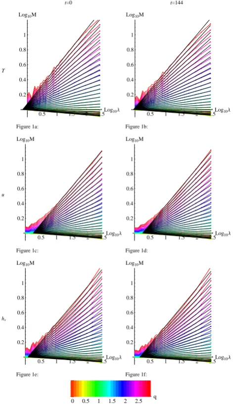
Figure 1 shows plots of log10Mq forT,u,hs for both the GEM analysis (t=0; Fig. 1a, c, e) and the t=144 h forecast (Fig. 1b, d, f) at 1000 mb, while Fig. 2 shows the correspond-ing plots (hr instead ofhs for GFS) for ERA40 (Fig. 2a, c, e) and GFS analysis datasets (Fig. 2b, d, f) at 1000 mb and Fig. 3 shows the moments of ufield at 700 mb for all datasets taken between±30◦(Fig. 3a, c, e) and±45◦latitude (Fig. 3b, d, f). Note that the 1000 mb fields are more influ-enced by the data – although with nontrivial effects where the topography is important – while the 700 mb fields are more representative of the free atmosphere. All the plots display the typical cascade “signature” – the converging straight lines predicted by Eq. (10). The regressions were performed by minimizing the deviations (Eq. 11, defined below) through a common intersection point over the range from the grid scale to 5000 km. Since we test the predictions of multiplica-tive cascade models, all lines were forced to pass through the same point (Eq. 10 withλ=λeff). Two remarkable fea-tures are: a) the cascades begin at an outer scale very close to the scale of the planet and b) up to≈5000 km the cas-cade structure is accurately followed. Note that Leff>Lref (=20 000 km) simply indicates that there is residual variabil-ity at planetary scales, whileLeff<Lrefindicates that it re-quires a certain range of scales for the scaling to become de-veloped.
To quantify the accuracy with which Eq. (10) is satisfied, we characterize the deviations using the mean absolute resid-uals for the statistical momentsMqof orderqfrom 0.0 to 2.0, for all points between the scale of the grid and 5000 km:
1=log10 Mq−K(q)log10(λ/λeff)
. (11)
To convert 1 to a percent deviation, δ=100(101−1)was used; we foundδ<±2% for all analyzed fields andδ<±1% for all initial analyses and short-range forecasts. This accu-racy is very close to those of the same moments of the visi-ble and IR radiances over the range 10–5000 km (≈±0.5%, Lovejoy et al., 2009a).
For the fields, the scaling extends from the grid size up to ∼5000–20 000 km. It is worth noting that the outer scales for these fields (∼8000–27 000 km) are approximately the same as the outer scales of the radiances (∼5000–32 000 km in Lovejoy et al., 2009a). We also mention that theC1’s are not too different from theC1’s for passive scalars (∼0.1) (Lilley et al., 2004). Similar results were found for the moments of the 2-D wind estimate of the energy flux.
t=0 t=144
T
0.5 1 1.5 2 2.5Log10l
0.2 0.4 0.6 0.8 1 Log10M
Figure 1a:
0.5 1 1.5 2 2.5Log10l
0.2 0.4 0.6 0.8 1 Log10M
Figure 1b:
u
0.5 1 1.5 2 2.5Log10l
0.2 0.4 0.6 0.8 1 Log10M
Figure 1c:
0.5 1 1.5 2 2.5Log10l
0.2 0.4 0.6 0.8 1 Log10M
Figure 1d:
hs
0.5 1 1.5 2 2.5Log10l
0.2 0.4 0.6 0.8 1 Log10M
Figure 1e:
0.5 1 1.5 2 2.5Log10l
0.2 0.4 0.6 0.8 1 Log10M
Figure 1f:
0 0.5 1 1.5 2 2.5 q
Fig. 1. Moments of fields for GEM at 1000 mb forq=0.0 to 2.9
(q>1.0: Log10Mq>0, monotonically increasing; q<1.0: Log10
Mq<0) in steps of 0.1,λ=Learth/L,Learth=20 000 km. Theqt h
-moment colour key is given at the bottom of the figure (q=0
(reddish-orange) toq=2.9 (red)). Left, at timet=0, on the right, the
144 h forecast; from top to bottom, temperature, east-west wind,
specific humidity, all between±30◦latitude. (a) temperature at
initialization; (b) temperature at 144hforecast; (c)uwind at
ini-tialization; (d)uwind at 144 h forecast; (e)hs at initialization; (f)
hsat 144 h forecast. For the parameters, refer to Table 2b.
we can also see that theK(q)“shape parameter” – the dif-ficult to estimate multifractal indexα– is roughly constant atα≈1.8±0.1. We examine the issue of the accuracy of this parametric representation, Eq. (1b), in Sect. 3.4. From Ta-ble 2a, we see that the scale by scale characterization of the intermittency near the mean (C1) has a tendency to decrease with altitude, this being somewhat amplified by a decrease in
the external scale (which decreases all the moments by the same factor). Interestingly, theC1values are very similar for the different fields (it is slightly larger for the humidity), al-though significantly, theC1are quite a bit larger than those measured by aircraft (Sect. 2.5 in Lovejoy et al., 2009b), also shown in the table.
Also in Table 2a is a comparison of aircraft estimates of the parameters from Lovejoy et al. (2009b) which included an in-depth evaluation of the optimum scale range (4–40 km) needed to avoid spurious aircraft effects. Since the aircraft fluxes were estimated in the scaling regime, we don’t expect the parameters to be identical to the dissipation range fluxes estimated here (see the discussion in Sect. 2). However, when the theoretical correction factor (assumingα=1.8) is used, the agreement is seen to be good (it is much improved). Note that the agreement is not expected to be perfect since Eq. (9) depends on an explicit identification of the conserved flux; while the argument is fairly robust for the velocity – as indi-cated – it is not so for the other quantities. In addition both the aircraft and model estimates will have some systematic biases so that our main point is that the results are plausibly consistent.
In order to estimate the parameter uncertainties, we calcu-lated them over subsets of the data for±30◦– each subset is about 1 month long – as indicated in the last row of Table 1. For all datasets, the maximum and minimum value ofαfor each subset in every dataset differ by less than 0.1 with the following exceptions: ERA40 hs 850 mbar (0.27), ERA40
hs 200 mbar (0.22). The maximum and minimum values of
C1 for each subset differ by less than 0.008 for GEM and GFS and less than 0.014 for ERA40. The maximum varia-tion in the estimates of log10λeffis less than 0.08 for GEM and GFS and less than 0.2 for ERA40 with the following ex-ceptions for ERA40: (u 850 mbar (0.2), T 200 mbar (0.2),
hs 850 mbar (0.3), hs 200 mbar (0.5)). For the most part, the deviations from the parameters estimated from 1 year of data are small, but it should not be surprising that there are occasional larger deviations because large amounts of data are needed to estimate parameters accurately for multifractal data.
Table 1. Comparison of various model parameters. The time step is the model integration time step. The last row indicates the size of the
subsets used to estimate the uncertainties (see the text).
Model GEM GFS ERA 40
Time step 22.5 7.5 30
(minutes)Tst
Model Spatial 0.25◦×0.3◦ 0.47◦×0.47◦ 1.125◦×1.125◦
resolution (grid size)
Spatial resolution of 0.6◦×0.6◦ 1◦×1◦ 1◦×1◦
the analysisLi
Number of vertical 28 64 60
levels
Number of realizations 505 1340 4384
in the sample
Time interval between 12 6 6
realizations (hours)
Size of dataset 25-25.5 days 30-30.5 days 1 month
subset (50–51 time steps) (120–122 time steps) (116–124 time steps)
Table 2a. Intercomparison of cascade parameters for the initial (t=0) fields for various fields at 1000, 700 mb. The triplets of values are for, ERA40 (denoted by “ERA”), GEM, GFS respectively. The aircraft estimates are from about 200 mb (the figure in parentheses is from
aircraft analyses (Lovejoy et al., 2009c, Table 3 forC1,α, Table 1 forLeff,δ), the second is corrected by the factor (3/2)α needed – at least
for the wind field – to estimate the dissipation scaleC1from the scaling rangeC1, see Eq. 9).
C1 α Leff(km) δ(%)
ERA GEM GFS ERA GEM GFS ERA GEM GFS ERA GEM GFS
T (1000) 0.113 0.125 0.142 1.94 1.64 1.72 21 900 25 800 28 000 0.31 0.27 0.59
T (700) 0.094 0.077 0.080 2.11 1.94 2.00 14 500 8300 8600 0.29 0.47 1.02
T (200) 0.080 0.080 0.065 1.93 1.88 1.85 12 100 10 700 7800 0.30 0.36 1.17
T (aircraft) (0.052), 0.107 1.78 5000 0.5
u(1000) 0.105 0.121 0.114 1.93 1.68 1.80 12 900 11 000 12 300 0.33 0.32 0.54
u(700) 0.096 0.104 0.082 1.93 1.86 1.87 12 000 11 000 9000 0.24 0.29 0.83
u(200) 0.075 0.085 0.073 1.92 1.85 1.89 15 900 16 300 9000 0.267 0.35 0.76
u(aircraft) (0.040), 0.088 1.94 25 000 0.8
hs,hr (1000) 0.121 0.109 0.128 2.03 1.81 1.86 19 800 15 900 21 700 0.33 0.51 0.46
hs,hr(700) 0.094 0.100 0.091 1.75 1.60 1.74 11 000 11 800 9000 0.26 0.37 0.46
hs,hr(200) 0.085 0.109 0.100 1.73 1.54 1.70 50 000 33 000 9700 0.47 0.56 0.64
h(aircraft) (0.040), 0.083 1.81 10 000 0.5
In Table 2c, we compare the cascade parameters calculated between±30◦and±45◦in an admittedly crude attempt to see if there are any detectable differences between the trop-ics and a region including the midlatitudes. A latitude effect might arise because of the importance of the Coriolis force in the midlatitudes which makes the large scale winds quasi-geostrophic. We find that the only notable difference is that the outer scale is systematically larger for the±45◦region. It could be noted that although we did not use equal area grids, the variation in grid size is still fairly small even at 45◦.
3.4 Universality and Levy collapse
Table 2b. An intercomparison of the 1000 mb fields, the triplets representing the parameter estimates for integrations oft=0, 48, 144 h.
C1 α Leff(km) δ(%)
0 h 48 h 144 h 0 h 48 h 144 h 0 h 48 h 144vh 0 h 48 h 144 h
T (GEM) 0.125 0.115 0.113 1.64 1.68 1.69 25 700 20 500 21 000 0.27 0.26 0.67
T (GFS) 0.142 0.138 1.72 1.71 27 900 26 000 0.59 0.60
u(GEM) 0.121 0.122 0.122 1.68 1.62 1.63 11 000 11 000 11 000 0.32 0.36 1.14
u(GFS) 0.114 0.107 1.80 1.84 12 300 11 200 0.54 0.64
hs(GEM) 0.109 0.106 0.107 1.81 1.80 1.80 15 900 13 800 13 500 0.51 0.49 1.54
hr (GFS) 0.128 0.128 1.86 1.81 21 700 20 900 0.46 0.46
Table 2c. An intercomparison of ranges of values of data in 700 mb fields between, pairs representing parameter estimates at analysis time
step for±30◦and±45◦. * The first two months were excluded because of corrupt data.
C1 α Leff(km) δ(%)
±30◦ ±45◦ ±30◦ ±45◦ ±30◦ ±45◦ ±30◦ ±45◦
T (ERA40) 0.094 0.091 2.11 2.11 14 500 21 400 0.288 0.274
T (GEM) 0.077 0.082 1.94 2.19 8300 17 000 0.47 0.36
T (GFS) 0.080 0.084 2.00 2.03 8600 11 100 1.03 0.88
u(ERA40) 0.096 0.094 1.93 1.90 12 000 14 000 0.239 0.225
u(GEM) 0.104 0.106 1.86 1.84 10 900 12 600 0.295 0.34
u(GFS)* 0.085 0.082 1.87 1.87 9000 10 100 0.83 0.69
hs(ERA40) 0.093 0.097 1.74 1.73 11 000 14 300 0.259 0.224
hs(GEM) 0.100 0.105 1.60 1.61 11 800 14 800 0.37 0.33
hr(GFS) 0.091 0.094 1.74 1.72 9000 9000 0.46 0.39
justify a two parameter (C1,α)regression. Since both pa-rameters have fairly simple interpretations (in terms of the closest monofractal approximation (C1)and the curvature of
K(q)nearq=1 (α)), the variation of these parameters with model type, integration time etc. can conveniently be used to characterize the variation of the cascade structure. However, we also argued that there are basic physical, mathematical reasons (essentially the existence of a kind of multiplicative central limit theorem) that make it plausible that the model outputs fall into special universality classes in which the ba-sic scale invariant exponentK(q)is given by Eq. (1b) char-acterized by just two parametersC1,α. In this section we explore the accuracy of Eq. (1b).
We must first note that even for perfect universal mul-tifractal processes, Eq. (1b) is only expected to be strictly valid for the “bare” cascade properties, i.e. those of an infi-nite ensemble of realizations of a cascade developed down to scaleL=Lref/λand then stopped. However, when analyzing the model output, we analyzed the “dressed” quantities, i.e. those obtained by degrading (by integrating) the resolution of a cascade developed to small scales (for the “bare”/”dressed” distinction see Schertzer and Lovejoy, 1987), and these were
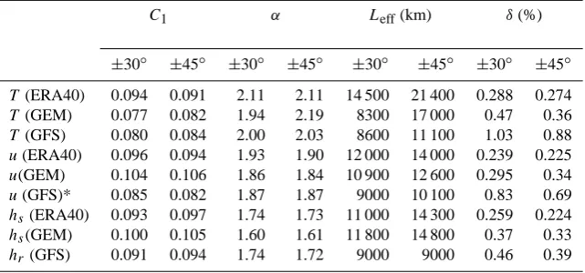
estimated using only a finite number of realizations. Both the bare/dressed distinction and the finite sample size give rise to (first or second order) “multifractal phase transitions” (Schertzer et al., 1993). This means that the measured (dressed) moments will only have the theoretical bare expo-nentK(q)for q below a critical moment qc beyond which there is a – multifractal phase transition – whereKbecomes asymptotically linear (a sample size-dependent effect corre-sponding to the domination of the statistics by the largest flux values present). In Fig. 4, using some representative compar-isons ofK(q)and the fits to the universal multifractal form (Eq. 1b), we see that the universal form is in fact very closely followed except for hints of linearity for someq≥qc>2. In fact forq<2, the deviations from the universal form are of the order±1− ±2%.
ERA40 GFS
T
0.5 1 1.5 2 Log10l
0.2 0.4 0.6 0.8 1 Log10M
Figure 2a:
0.5 1 1.5 2 Log10l
0.2 0.4 0.6 0.8 1 Log10M
Figure 2b:
u
0.5 1 1.5 2 Log10l
0.2 0.4 0.6 0.8 1 Log10M
Figure 2c:
0.5 1 1.5 2 Log10l
0.2 0.4 0.6 0.8 1 Log10M
Figure 2d:
hs, hr
0.5 1 1.5 2 Log10l
0.2 0.4 0.6 0.8 1 Log10M
Figure 2e:
0.5 1 1.5 2 Log10l
0.2 0.4 0.6 0.8 1 Log10M
Figure 2f:
0 0.5 1 1.5 2 2.5 q
Fig. 2. Moments of the ERA40, GFS (t=0) fields at 1000 mbar
for q=0.0 to 2.9 (q>1.0: Log10Mq>0, monotonically
in-creasing; q<1.0: Log10Mq<0) in steps of 0.1, λ=Learth/L,
Learth=20 000 km. Theqt h-moment colour key is given at the
bot-tom of the figure (q=0 (reddish-orange) toq=2.9 (red)). On the
left, ERA 40, on the right, the GFS, top to bottom: temperature,
east-west wind, and humidity, between±30◦latitude. (a) ERA40
temperature; (b) GFS analysis temperature; (c) ERA40uwind; (d)
GFS analysisuwind; (e) ERA40hs; (f) GFS analysishr. For the
corresponding parameters, refer to Table 2a.
theoretical K(q) for (say) C1=1, i.e. by dividing by (qα−q)/(α−1). IfMqdoes indeed follow Eq. (1a) and (1b) with parametersC1,α, then can define the “collapsed mo-ments”:
Mq0 = Mq
(α−1) qα−q
±30º ±45º
ERA
0.5 1 1.5 2 Log10l
0.2 0.4 0.6 0.8 1 Log10M
Figure 3a:
0.5 1 1.5 2 Log10l
0.2 0.4 0.6 0.8 1 Log10M
Figure 3b:
GEM
0.5 1 1.5 2 2.5Log10l
0.2 0.4 0.6 0.8 1 Log10M
Figure 3c:
0.5 1 1.5 2 2.5Log10l
0.2 0.4 0.6 0.8 1 Log10M
Figure 3d:
GFS
0.5 1 1.5 2 Log10l
0.2 0.4 0.6 0.8 1 Log10M
Figure 3e:
0.5 1 1.5 2 Log10l
0.2 0.4 0.6 0.8 1 Log10M
Figure 3f:
0 0.5 1 1.5 2 2.5 q
Fig. 3. Moments ofufields analysis time step at 700 mbar forq=0.0
to 2.9 (q>1.0: Log10Mq>0, monotonically increasing; q<1.0:
Log10Mq<0) in steps of 0.1,λ=Learth/L,Learth=20 000 km. The
qt h-moment colour key is given at the bottom of the figure (q=0
(reddish-orange) to q=2.9 (red)). The left column are analyses
between±30◦latitude, the right hand between±45◦, top to
bot-tom, ERA 40 (denoted by “ERA”), GEM (t=0), GFS (t=0). (a)
ERA40 between±30◦latitude; (b) ERA40 between±45◦latitude;
(c) GEM between±30◦latitude; (d) GEM between±45◦latitude;
(e) GFS between±30◦ latitude; (f) GFS±45◦latitude. For the corresponding parameters, refer to Table 2c.
which for universal multifractals, withq<qcyields:
Mq0 =λC1;
0.5 1 1.5 2 2.5 q 0.1
0.2 0.3 0.4 0.5 KHqL
a) b)
c)
0.5 1 1.5 2 2.5 q
0.1 0.2 0.3 0.4 0.5 0.6 KHqL
0.5 1 1.5 2 2.5 q
0.1 0.2 0.3 0.4 0.5 0.6 KHqL
Fig. 4.K(q)forT at 1000 mb 00:00 h timestep between±30◦for
(a) GEM, (b) ERA40, (c) GFS. Dots are the calculated values for
K(q)at eachq(0.0 to 2.9). Solid lines are fits for (a)C1=0.125,
α=1.64 (b), C1=0.113, α=1.94 and (c), C1=0.142, α=1.72.
No-tice the linear deviation of dots from the curves forq>2, which
is indicative of a multifractal phase transition caused by the finite sample size.
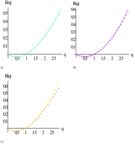
collapsed lines) as well as the log-Levy nature of the gener-ator – by the thinness of the collection of lines i.e. how well at a given scale the different moments collapse, how well they follow the functional form (qα−q). If the flux follows Eq. (1b), it implies that the generator of the cascade (log flux) is a Levy variable, indexα, so that we may call this a “Levy collapse”. The “thinness” can be quantified at each scaleλ
by the relative standard deviation ofMq’ as functions ofq:
δ=100 LogMλ0−LogMλ0
2 !1/2
/LogMλ0
(the overbars indicate averaging with respect to the q values). In Figs. 5, 6, 7 we see that the collapse for the different mod-els, different fields, different altitudes, different forecast pe-riods is very good, and this even out to scales where the scal-ing is not so well respected. The right hand column shows for eachλthe relative root mean square deviation (=δ) of the collapsed curves. For all scales the variations in logMq0 are of the order±2–±10% about the mean values (Fig. 5, 6, 7). The main exceptions are at the single small scale (largestλ)
point which is presumably a finite size effect associated with the spatial discretization of the grid at the single pixel scale, as well as the occasionally deviations>10% at the largest
scales (where the number of independent structures sampled is lowest and the statistics are poorest). In Fig. 6, we show the systematic variation of the collapse with altitude, Fig. 7 with forecast time. The Levy collapse presentation has the attractive feature of allowing us to superpose the correspond-ing fields of the different models, thus makcorrespond-ing succinct inter model comparisons possible.
In the previous section, we noted that for all the fields, the regression estimates of α were close to the value 1.8. Looking more closely, we find overall that for a given field, all altitudes have roughly the sameα. There are some fea-tures worth mentioning; for example, for GEM, α is con-sistently about 0.20 smaller than ERA40 for hs, while u andT at 1000 mb haveα∼1.65 for GEM compared to 1.94 for ERA40 therefore show differences mostly not too differ-ent (0.10 greater) for the higher altitudes. The GFS model typically shows intermediate results between the two other datasets.
In order to see howαvaries for the same field but at differ-ent altitudes we calculated the “reduced momdiffer-ents,”M1/C1
q , withC1 estimated numerically from C1=K’(1). This sep-arates the changes due to the mean intermittency C1 from changes in the shape due to differentLeff’s andα’s. If the reduced moments are equal, then the only difference is in the mean intermittency (C1)parameter. Figure 6 shows the re-duced moments foru,T,hs for GEM and ERA40 (the 48 h GEM forecast was very similar to the analysis) forq=0.5 and
q=2. We see that the curves – including the small deviations from linearity at large scales (smallλ)are very close so that variations inC1do indeed capture much of the field to field variability, variations in the value ofα andLeff are indeed small.
4 Conclusions
0.5 1 1.5 2 2.5Log10l 0.05
0.1 0.15 0.2 0.25 0.3 Log10M'
a)
0.5 1 1.5 2 2.5Log10l 2
4 6 8 10 12 14
d%
b)
0.5 1 1.5 2 2.5Log10l 0.05
0.1 0.15 0.2 0.25 0.3 Log10M'
c)
0.5 1 1.5 2 2.5Log10l 2
4 6 8 10 12 14
d%
d)
0.5 1 1.5 2 2.5Log10l 0.05
0.1 0.15 0.2 0.25 0.3 Log10M'
e)
0.5 1 1.5 2 2.5Log10l 2
4 6 8 10 12 14
d%
f)
0.5 1 1.5 2 2.5Log10l 0.05
0.1 0.15 0.2 0.25 0.3 Log10M'
g)
0.5 1 1.5 2 2.5Log10l 2
4 6 8 10 12 14
d%
h)
Fig. 5. Levy Collapse Diagrams, showing log10Mq’=
(α−1)Log10Mq/ qα−q, showing moments, q=0.1,
0.2, 0.3, . . . 2.0, (excluding q=1.0) for each diagram
(left hand side), and their corresponding deviations
δ=100 LogMλ0−LogMλ0
2 !1/2
/LogMλ0 as a function of
scale (right hand size). If at a given scaleλ, the curves overlap
for allqit implies that the generator (log) of the process is a Levy
random variable with corresponding indexα; the “collapsed” log
moments=C1logλ(independent of q). In what follows, the red
curves are GEM, green are ERA40, blue are GFS. (a)u700 mbar:
GEM (red, α=1.9), ERA40 (green, α=2.0), GFS (blue, α=1.85);
(b) percentage deviation of moments corresponding to (a); (c)T
1000 mbar: GEM (red, =1.7), ERA40 (green,α=1.95), GFS (blue,
α=1.75); (d) percentage deviation of moments corresponding
to (c); (e) T 700 mbar: GEM (red, α=2.05), ERA40 (green,
α=2.2), GFS (blue,α=2.15); (f) percentage deviation of moments
corresponding to (e); (g) 700 mbarhs: GEM (red,α=1.65), ERA40
(green,α=1.8),hr GFS (blue,α=1.8); (h) percentage deviation of
moments corresponding to (g). The slope of the lines isC1and the
horizontal intercept is the outer scale given in Table 2.
Fig. 6. More Levy collapse curves (left), here as a function of
al-titude, and their corresponding deviationsδ(right) as a function of
scale (a) GEM collapse curvesu: 1000 mb (red,α=1.7) , 700 mb
(green, α=1.9), 200 mb (blue, α=1.85); (b) percentage deviation
as a function of scale, corresponding to (a); (c)hs ERA40:
col-lapse curves 1000 mb (red,α=2.05), 700 mb (green,α=1.8), 200 mb
(blue,α=1.73); (d) percentage deviation as a function of scale,
cor-responding to (c). The slope of the lines isC1and the horizontal
intercept is the outer scale given in Table 2.
Fig. 7. More Levy collapse curves, (left) here as a function of
fore-cast time, and their corresponding deviationsδas a function of scale
(right) (a) GEMhs850 mb:t=0 h (red,α=1.73,C1=0.90,λ=0.31),
t=48 h (green,α=1.77,C1=0.088,λ=0.27),t=144 h (blue,α=1.78,
C1=0.094,λ=0.26); (b) percentage deviation as a function of scale,
corresponding to a; (c)hs ERA40 collapse curves: 1000 mb (red,
α=2.00), 700 mb (green, α=1.97); (d) percentage deviation as a
function of scale, corresponding to (c). The slope of the lines is
C1and the horizontal intercept is the outer scale, which is given in
Table 2 for (b). Note that theαvalue may vary slightly depending
consequence is that there is no currently accepted turbulence interpretation of the model statistics.
However starting in the 1960’s – in order to help under-stand intermittency, – precise, explicit multiplicative cas-cades models were developed. These phenomenological models are designed to reproduce some of the symmetries of the governing dynamical equations, specifically the scale by scale conservation of turbulent fluxes, the scale invariance symmetries of the dynamics and localness in Fourier space (so that interactions are primarily between structures of simi-lar size). An advantage of directly exploiting the scale invari-ance is that no specific a priori assumptions need to be made about either isotropy or about the physical nature of the cas-cade quantity; the (generally anisotropic) scale symmetries play a crucial role. It is now understood that the implica-tions are quite generic – they are insensitive to many details so that the statistics are expected to obey the basic prediction of multiplicative cascades Eq. (1a). In addition, due to the existence of stable attractive universality classes (a kind of multiplicative central limit theorem), there is an even more precise prediction – that the exponentK(q)should depend only on two basic parameters (Eq. 1b).
Using (now standard) data analysis techniques, we demon-strate that three leading numerical models of the atmosphere accurately follow the predictions of multiplicative cascade models, including one (the reanalysis ERA 40) where ex-tensive analysis of the classical (isotropic turbulence) ap-proach failed to follow the predictions of the isotropic the-ories (Straus and Ditlevsen, 1999). In retrospect, it is fortu-nate that the models nearly perfectly follow the cascade pre-dictions because an increasing number of analyses of empir-ical atmospheric data find that the atmosphere also has a cas-cade structure, so that the statistics of the data and numerical models are at least in qualitative (structural) agreement. The cascade structure of the intialisation fields makes it possible that the results are at least partially imposed by the constraint that they are near the (cascade-like) data att=0. However, the forecasts – both short (48 h) and medium-range (144 h) – show that the model statistics are little changed although there is a small increase in the residuals,δ. This suggests – but does not prove – that if the same models were run in “climate-mode” – i.e. for very long integrations – that they would maintain a cascade structure.
Over the period where numerical and multiplicative cas-cade models were developed in parallel, they have sometimes seemed irreconcilable – if only because the former are de-terministic with strong scale truncations, whereas the latter are stochastic over arbitrarily wide ranges of scale. How-ever in the last 15 years, with the development of “ensemble” forecasting (e.g., Zoth and Kalnay, 1993), there has been a revolution in attitudes about forecasting; it is now increas-ingly accepted that the goal is no longer a deterministic fore-cast of the weather (or climate) but rather the production of a distribution of possible future atmospheric states includ-ing their relative probabilities: today the aim is a
stochas-Fig. 8. “Reduced” C1-normalized moments (Mq1/C1) between
±30◦latitude of orderq=0.5 and 2 (bottom and top, respectively).
Moments for ERA40u(teal), ERA40T (cyan), ERA40hs (blue),
GEMu(orange), GEMT (lime), GEMhs (green), GFSu
(pur-ple), GFST (magenta), GFS hr (red), and reference lines for a
cascade (black) withLeff=11 200 km. The solid coloured lines are
the mean value of the moments of a field over all pressure levels (1000, 850, 700, 500, 200 mb), while the error bars show the spread (maximum/minimum) in values for different altitudes.
tic one. At the moment, this goal can only be achieved by a nontrivial marriage between the deterministic models and stochasticity, which is currently artificially introduced via various methods of generating initial conditions (e.g. “en-semble breeding”, see Corazza et al., 2003). Other ad hoc attempts such as Buizza et al. (1999) and Palmer (2001) to introduce the required stochasticity include attempts at sub-grid “stochastic parameterization”. With the findings of this paper that cascades accurately describe the stochastic struc-ture of the equations, several new avenues for modelling ap-pear. The stochastic parameterization in this case can be used to properly implement an ensemble forecast – so differences in each member of the ensemble appear because of changes in the fields due to the stochastic parameterization. In the short term, using the cascades as theoretically “clean” sub-grid parameterizations is promising, while in the medium to long term, quite new more direct purely stochastic forecast-ing techniques will be possible by exploitforecast-ing the long range memory implicit in the cascade structures as mentioned in Scherzter and Lovejoy (2004).
Acknowledgements. We would like to acknowledge NSERC for
Jonathan Stolle’s scholarship support as well as Michel Bourqui, Andrew Ryzkhov, and Charles Lin for their helpful discussions
and technical expertise. The analysis of GEM data was based
on Environment Canada data and the ERA40 data developed by the ECMWF was obtained through UCAR. We also thank anonymous referees of Phys. Rev. Lett. and Physica A for some of their comments. This project did not receive any specific funding.
Edited by: A. Turiel
References
Biferale, L.: Shell models of energy cascade
tur-bulence, Annu. Rev. Fluid Mech., 35, 441–468,
doi:10.1146/annurev.fluid.35.101101.161122, 2003.
Blender, R. and Fraedrich, K.: Long time memory in global warming simulations, Geophys. Res. Lett., 30, 1769–1772, doi:10.1029/2003GL017666, 2003.
Boer, G. J. and Shepherd, T. G.: Large-scale two-dimensional tur-bulence in the atmosphere, J. Atmos. Sci., 40, 164–184, 1983. Buizza, R., Miller, M., and Palmer, T. N.: Stochastic
representa-tion of model uncertainties in the ECMWF Ensemble Predicrepresenta-tion System, Q. J. Roy. Meteor. Soc., 125, 2887–2908, 1999. Chigirinskaya, H. Y. and Schertzer, D.: Cascade of scaling
gyro-scopes: Lie stucture, universal multifractals and self-organized criticality in turbulence, in: Stochastic Models in Geosystems, edited by: Molchanov, S. A. and Woyczynski, W. A., Springer, New York, 57–81, 1997.
Chigirinskaya, Y., Schertzer, D., and. Lovejoy, S: An alternative to shell-models, more complete and yet simple models of intermit-tency, in: European Turbulence 7, edited by: Frisch, U., Kluwer Academic Press, Dordrecht, 263–266, 1998.
Cho, J. and Lindborg, E.: Horizontal velocity structure functions in the upper troposphere and lower stratosphere I: Observations, J. Geophys. Res., 106,, 10223–10232, 2001.
CMC Global Data Assimilation System (DAS), online
avail-able at: http://www.meted.ucar.edu/nwp/pcu2/GEMglobal/
gemglobassim.htm, last access: 22 July 2009.
Corazza, M., Kalnay, E., Patil, D. J., Yang, S.-C., Morss, R., Cai, M., Szunyogh, I., Hunt, B. R., and Yorke, J. A.: Use of the breed-ing technique to estimate the structure of the analysis “errors of the day”, Nonlin. Processes Geophys., 10, 233–243, 2003, http://www.nonlin-processes-geophys.net/10/233/2003/. Cˆote, J., Desmarais, J.-D., Gravel, S., Methot, A., Patoine, A.,
Roch, M., and Staniforth, A.: The operational CMC-MRB global environmental multiscale (GEM) model. Part II: Results, Mon. Weather Rev., 126, 1397–1418, 1998.
Cˆote, J., Gravel, S., Methot, A., Patoine, A., Roch, M., and Stan-iforth, A.: The operational CMC-MRB global environmental multiscale (GEM) model. Part I: Design considerations and for-mulation, Mon. Weather Rev., 126, 1373–1395, 1998.
Dewan, E. and Good, R.: Saturation and the universal spectrum for vertical profiles of horizontal scalar winds in the atmosphere, J. Geophys. Res., 91, 2742–2748, 1986.
Dewan, E.: Saturated-cascade similitude theory of gravity wave spectra, J. Geophys. Res., 102, 29799–29817, 1997.
Fraedrich, K. and Blender, R.: Scaling of Atmosphere
and Ocean Temperature Correlations in Observations
and Climate Models, Phys. Rev. Lett., 90, 108501,
doi:10.1103/PhysRevLett.90.108501, 2003.
Frisch, U., Kurien, S., Pandit, R., Pauls, W., Ray, S. S., Wirth, A., and Zhu, J.-Z.: Hyperviscosity, Galerkin Truncation, and Bottlenecks in Turbulence, Phys. Rev. Lett., 101, 144501, doi:0.1103/PhysRevLett.101.144501, 2008.
Gage, K. S. and Nastrom, G. D.: Theoretical interpretation of atmo-spheric wavenumber spectra of wind and temperature observed by commercial aircraft during GASP, J. Atmos. Sci., 43, 729– 740, 1986.
Gagnon, J.-S., Lovejoy, S., and Schertzer, D.: Multifractal earth topography, Nonlin. Processes Geophys., 13, 541–570, 2006,
http://www.nonlin-processes-geophys.net/13/541/2006/. Gardner, C.: Diffusive filtering theory of gravity wave spectra in the
atmosphere, J. Geophys. Res., 99, 20601–20622, 1994. Hamilton, K., Takahashi, Y. O., and Ohfuchi, W.: Mesoscale
spec-trum of atmospheric motions investigated in a very fine resolu-tion global general cirucularesolu-tion model, J. Geophys. Res., 113, D18110, doi:18110.11029/12008JD009785, 2008.
Hamilton, K.: Numerical Resolution and Modeling of the Global Atmospheric Circulation: A Review of Our Current Understand-ing and OutstandUnderstand-ing Issues in High Resolution Numerical Mod-elling of the Atmosphere and Ocean, edited by: Hamilton, K. and Ohfuchi, W., 7–27, 2007.
Haugen, N. E. L. and Brandenburg, A.: Inertial range scaling in numerical turbulence with hyperviscosity, Phys. Rev. E, 026405, doi:10.1103/PhysRevE.70.026405, 2004.
High-resolution CMC GRIB dataset, online available at: http: //www.weatheroffice.gc.ca/grib/High-resolution GRIB e.html, last access: 6 February 2009.
Kaneda, Y., Ishihara, T., Yokokawa M., Itakura K., and Uno, A.: Energy dissipation rate and energy spectrum in high resolution direct numerical simulations of turbulence in a periodic box, Phys. Fluids, 15, L21–L24, doi:10.1063/1.1539855, 2003. Kolmogorov, A. N.: Local structure of turbulence in an
incompress-ible liquid for very large Reynolds numbers, Proc. Acad. Sci. USSR. Geochem Sect., 30, 299–303, 1941.
Landau, L. D. and Lifshitz, E. M.: Fluid Mechanics, 2nd Ed., Course of Theoretical Physics, Vol. 6, Pergamon, Oxford, 1987. Lilley, M., Lovejoy, S., Strawbridge, K., and Schertzer D.: 23/9 dimensional anisotropic scaling of passive admixtures
using lidar aerosol data, Phys. Rev. E, 70, 036307-1,
doi:10.1103/PhysRevE.70.036307, 2004.
Lilley, M. Lovejoy, S., Strawbridge, K. B., Schertzer, D., and Rad-kevich, A.: Scaling turbulent atmospheric stratification, Part II: spatial stratification and intermittency from lidar data, Q. J. Roy. Meteor. Soc. 134, 301–315, doi:10.1002/qj.1202, 2008. Lindborg, E.: Can the atmospheric kinetic energy spectrum be
ex-plained by two-dimensional turbulence?, J. Fluid Mech., 388, 259–288, 1999.
Lovejoy, S., Schertzer, D., and Stanway, J. D.: Direct Evidence of planetary scale atmospheric cascade dynamics, Phys. Rev. Lett. 86, 5200–5203, 2001.
Lovejoy, S. Schertzer, D., and Tuck, A. F.: Fractal aircraft trajec-tories and nonclassical turbulent exponents, Phys. Rev. E, 70, 036306-1, doi:0.1103/PhysRevE.70.03630, 2004.
Lovejoy, S., Hovde, S., Tuck, A., and Schertzer, D.: Is isotropic turbulence relevant in the atmosphere?, Geophys. Res. Lett., 34, L14802, doi:10.1029/2007GL029359, 2007.
Lovejoy, S., Schertzer, D., Lilley, M., Strawbridge, K., and Rad-kevich, A.: Scaling turbulent atmospheric stratification. I: tur-bulence and waves, Q. J. Roy. Meteor. Soc., 134, 277–300, doi:10.1002/qj.1201, 2008.
Lovejoy, S., Schertzer, D., Allaire, V., Bourgeois, T., King,
S., Pinel, J., and Stolle, J.: Atmospheric complexity or
scale by scale simplicity?, Geophys. Res. Lett., 36, L01801, doi:01810.01029/02008GL035863, 2009a.
Lovejoy, S. and Schertzer, D.: Towards a new synthesis for atmo-spheric dynamics: space-time cascades, Atmos. Res., in press, 2009.
structure of the atmosphere from aircraft measurements, J. Geo-phys. Res., submitted, 2009b.
Lovejoy, S., Tuck, A. F., Schertzer, D., and Hovde, S. J.: Reinter-preting aircraft measurements in anisotropic scaling turbulence, Atmos. Chem. Phys., 9, 5007–5025, 2009c,
http://www.atmos-chem-phys.net/9/5007/2009/.
Lovejoy, S., Tuck, A. F., Hovde S. J., and Schertzer D.: The vertical cascade structure of the atmosphere and multifrac-tal drop sonde outages, J. Geophys. Res., 114, D07111, doi:10.1029/2008JD010651, 2009d.
Mandelbrot, B. B.: Intermittent turbulence in self-similar cascades: divergence of high moments and dimension of the carrier, J. Fluid Mech., 62, 331–358, 1974.
Monin, A. S. and Yaglom, A. M.: Statistical Fluid Mechanics, MIT Press, Boston, 1975.
NCEP Office Note 442: The GFS atmospheric model, online avail-able at: http://www.emc.ncep.noaa.gov/officenotes/newernotes/ on442.pdf, last access: 6 February 2009.
Novikov, E. A. and Stewart, R.: Intermittency of turbulence
and spectrum of fluctuations in energy dissipation, Izvestiia Akademii nauk SSSR, Seriia Geofizicheskaia, 3, 408–412, 1964. Okamoto, K. and Derber, J.: Assimilation of SSM/I radiance in the NCEP global data assimilation system, Mon. Weather Rev., doi: 10.1175/MWR3205.1, 2006.
Orszag, S. A. and Patterson, G. S.: Numerical simulation of three-dimensional homogenous Turbulence, Phys. Rev. Lett., 28, 76– 79, 1972.
Parisi, G. and Frisch, U.: A multifractal model of intermittency, in: Turbulence and predictability in geophysical fluid dynamics and climate dynamics, edited by: Ghil, M., Benzi, R., and Parisi, G., Amsterdam, Netherlands, 84–88, 1985.
Palmer, T. N.: A nonlinear dynamical perspective on model error: A proposal for non-local stochastic-dynamic parametrization in weather and climate prediction models, Q. J. Roy. Meteor. Soc., 127, 279–304, 2001.
Richardson, L. F.: Weather Prediction by Numerical Process, Cam-bridge University Press, CamCam-bridge, United Kingdom, 1922, re-published by Dover, New York, 1965.
Richardson, L. F.: Atmospheric diffusion shown on a distance-neighbour graph, Proc. Roy. Soc. Lond. A Mat., 110, 709–737, 1926.
Royer, J. F., Biaou, A., Chauvin, F., Schertzer, D., and Lovejoy, S.: Multifractal analysis of the evolution of simulated precipita-tion over France in a climate scenario, Comptes Rendues Geo-physiques, 340, 431–440, 2008.
Schertzer, D. and Lovejoy, S.: The dimension and intermittency of atmospheric dynamics, in: Turbulent Shear Flow 4 7, edited by: Launder, B., Springer, Berlin, 1985.
Schertzer, D. and Lovejoy, S.: Physical modeling and analysis of rain and clouds by anisotropic scaling of multiplicative pro-cesses, J. Geophys. Res., 92, 9692–9714, 1987.
Schertzer, D. and Lovejoy, S.: Uncertainty and Predictability
in Geophysics: Chaos and Multifractal Insights, in: State of the Planet, Frontiers and Challenges in Geophysics, edited by: Sparks, R. S. J. and Hawkesworth, C. J., AGU, Washington, 317– 334, 2004.
Schertzer, D., Lovejoy, S., and Lavall´ee, D.: Generic multifractal phase transitions and self-organized criticality in Cellular au-tomata: prospects, in: Astronomy and astrophysics, edited by: Perdang J. M. and Lejeune, A., World Scientific, 216–227, 1993. Sela, J. G.: The NMC spectral model, NOAA technical report
NWS-30, 1982.
Sela, J. G.: The new NMC operational spectral model, in: Eighth Conference on Numerical Weather Prediction, Baltimore, Mary-land, 22–26 February 1988.
Steinberg, H. L., Wiin-Nielsen, A., and Yang C.-H.: On nonlinear cascades in atmospheric flows, J. Geophys. Res. 76, 8629–8640, 1971.
Stolle, J.: A spatial and temporal stochastic cascade analysis of me-teorological models and reanalyses, McGill University, Canada, 2009.
Stolle, J., Lovejoy, S., and Scherzter, D.: The temporal cascade structure and space-time relations for reanalyses and Global Cir-culation models, in preparation, 2009.
Straus, D. M. and Ditlevsen, P.: Two dimensional turbulence prop-erties of the ECMWF, Tellus, 51A, 749–772, 1999.
Syroka, J. and Toumi, R.: Scaling and persistence in observed and modelled surface temperature, Geophys. Res. Lett., 28, 3255– 3255, 2001.
Toth, Z. and Kalnay, E.: Ensemble forecasting at NMC: the gen-eration of perturbations, B. Am. Meteorol. Soc., 74, 2317–2330, 1993.
Uppala, S. M., Kallberg, P. W., Simmons, A. J., Andrae, U., Da Costa Bechtold, V., Fiorino, M., Gibson, J. K., Haseler, J., Her-nandez, A., Kelly, G. A., Li, X., Onogi, K., Sarinen, S., Sokka, N., Allan, R. P., Anderson, E., Arpe, K., Balmaseda, M. A., Beljaars, A. C. M., Van de Berg, L., Bidloti, J., Bormann, N., Caires, S., Chevallier, F., Dethof, A., Dragosavac, M., Fisher, M., Fuentes, M., Hagemann, S., Holm, E., Hoskins, B. J., Isak-sen, L., JansIsak-sen, P. A. E. M., Jenne, R., McNally, A. P., Mahfouf, J.-F., Morcrette, J.-J., Rayner, N. A., Saunders, R. W., SIMON, P., Sterl, A., Trenberth, K. E., Untch, A., Vasiljevic, D., Viterbo, P., and Woollen, J.: The ERA40 re-analysis, Q. J. Roy. Meteor. Soc., 131, 2961–3012, doi:10.1256/qj.04.176, 2005.
Van Zandt, T. E.: A universal spectrum of buoyancy waves in the atmosphere, Geophys. Res. Lett., 9, 575–578, 1982.
Vincent, A. and Meneguzzi, M.: The spatial structure and statistical properties of homogeneous turbulence, J. Fluid Mech., 225, 1– 20, 1991.
Yaglom, A. M.: The influence of fluctuations in energy dissipation on the shape of turbulence characteristics in the inertial interval, Soviet Physics – Doklady., 2, 26–29, 1966.
Yokokawa, M., Itakura, K., Uno, A., Ishihara, T., and Kaneda, Y.: 16.4-Tflops Direct Numerical Simulation of Turbulence by a Fourier Spectral Method on the Earth Simulator, in: SC2002, Baltimore, USA, 16–22 November, online available at: