Comparisons of Experimental and Simulated Velocity Fields in Membrane Module Spacers

Keywords

Highlights

Abstract

Graphical abstract

283

Research Paper

Received 2019-01-12 Revised 2019-04-07 Accepted 2019-04-09 Available online 2019-04-09

Spiral wound module Spacer

Computational fluid dynamics Particle image velocimetry

• Good quantitative agreement between experiment and simulation for

velocities in spacer filled channels

• First comparison of all three velocity components presented

• Results support use of computational fluid dynamics for spacer

design

Comparisons of Experimental and Simulated Velocity Fields in Membrane Module Spacers

Chemical Engineering Department, The University of Toledo, 2801 W. Bancroft, Toledo, OH 43606, United States

Ravikumar Gogar, Ghazaleh Vaseghi, Glenn Lipscomb

Article info

© 2019 MPRL. All rights reserved.

* Corresponding author at: Phone: +1 419 530 8080; fax: +1 419 530 8086 E-mail address: glenn.lipscomb@utoledo.edu (G. Lipscomb)

DOI: 10.22079/JMSR.2019.101683.1242 1. Introduction

Spiral wound modules (SWM) are used widely in the chemical industry for gas separation and water purification. Figure 1 illustrates the placement of

feed and permeate spacers between alternate membrane layers in a module to create flow channels and provide mechanical support to the membranes [1]. Conventional spacers commonly are mesh-like structures of layered or woven cylindrical filaments as shown in Figure 2. Feed spacers disrupt the flow in the feed channel and can thereby improve mixing, minimize concentration

polarization, reduce fouling, and enhance mass transfer rates [2]. However,

the improvement in mixing and mass transfer comes at the cost of increased

pressure drop. The extent of mixing and pressure drop is governed by spacer geometric parameters, such as filament shape (typically cylindrical as illustrated

in Figure 2), filament thickness, filament spacing, angle between filaments, and filament angle relative to the nominal flow direction (x direction). Thus, the

efficiency of a membrane module is highly dependent on spacer geometry and the flow pattern it creates in the flow channel.

The spacer geometric parameters illustrated in Figure 2 can be varied to

optimize the performance of a module by changing the trade-off between

mixing and pressure drop [3]. To optimize spacer design, it is important to evaluate the fluid flow pattern in the spacer-filled channel. Common techniques to study fluid flow are (1) Computational Fluid Dynamics (CFD) – numerically solving the conservation of momentum and mass equations for given boundary and initial conditions and (2) Flow visualization – monitoring and analyzing the motion of tracer particles in the flow channel or using magnetic resonance imaging. CFD offers significant time- and cost-savings as spacer geometric parameters and flow conditions can be varied easily. However, to use CFD as a tool to study flow behavior it is important to

Journal of Membrane Science & Research

journal homepage: www.msrjournal.com

Spacers are used in spiral wound and plate and frame membrane modules to create flow channels between adjacent membrane layers and mix fluid within the flow channel. Flow through the spacer has a significant beneficial impact on mixing and resulting mass transfer rates but is accompanied by an undesirable increase in pressure drop. Computational Fluid Dynamics (CFD) is a common tool used to evaluate the effect of spacer design on fluid flow. While numerous theoretical studies are reported in the literature, confirmation of simulation results through experimental velocity field measurements is limited. Comparisons of CFD simulations with experimental velocity measurements using Particle Image Velocimetry (PIV) for traditional symmetric diamond and asymmetric spacer designs and a novel static mixing spacer design are presented. The results include comparisons of the two velocity components in planes parallel to the flow channel walls for the diamond and asymmetric spacer as well as the first reported comparisons of all three velocity components for the static mixing spacer. The results indicate good agreement between theory and experiment and help validate the use of CFD for spacer design.

validate simulations with experiments. Particle Image Velocimetry (PIV) is one such non-invasive experimental technique for visualization and measurement of flow behavior.

Fimbres-Weihs et al. [4] reported a comprehensive review of CFD studies in spacer-filled channels. More recent summaries also are available [5-7]. The reader is referred to these reviews of the vast literature on simulation for detailed discussions on different simulation approaches as the focus of this work is on experimental measurements of velocity for which the literature is much more limited.

The lack of experimental studies to validate simulations was highlighted. One of the first flow-visualization studies in a spacer-filled channel was conducted by Kang et al. [8] They investigated laminar flow in a spacer-filled channel by monitoring the motion of a tracer. Kim et al. [9] conducted flow-visualization studies using an ink tracer. They concluded that as the filament angle increases, the effectiveness of a spacer as a turbulence promoter also increases. Da Costa et al. [10] used dye injection to visualize the flow. A zig-zag flow pattern and changes in the bulk fluid flow direction were suggested by their still photographs of the moving fluid in the flow channel. The spread of dye was faster in high-angle spacers and angle was identified as an important parameter in spacer design. A similar zig-zag pattern was observed by Zimmerer et al. [11] in enlarged spacers using ammonia as a tracer. Karode et al. [12] conducted CFD simulations to obtain the velocity field within symmetric and asymmetric spacer-filled channels. They challenged the conclusion of Da Costa et al. [10] about the change in bulk fluid velocity. They observed that the bulk fluid flow was predominantly parallel to the filaments. Changes in direction occur only near the intersection of spacer filaments. The changes in fluid flow direction were less pronounced in the asymmetric spacer than in the symmetric spacer due to the differences in filament orientation. Cao et al. [13] conducted CFD simulations to obtain velocity profiles for various positions of cylindrical spacer filaments within the flow channel. Simulations were validated with comparisons of experimental and theoretical values for pressure drop. Saeed et al. [3] conducted 3D-simulations in rhombus-like spacers at various flow angles to obtain velocity fields. An increase in velocity was observed in the regions of filament cross-over. Neal et al. [14] used direct observation through the membrane to study particle deposition and flux enhancement using latex beads for various spacer orientations. Gimmelshtein et al. [15] investigated the flow in a rhombus-like spacer using 2D-PIV. Velocity profiles and mixing intensity were determined for a range of Reynolds numbers. The experimental results indicated that changes in flow direction occur near the spacer filaments. The thickness of the spacer used was about 20 % less than the flow channel height contrary to the more common use of spacers of comparable thickness. This created a region in the flow channel within which the spacer

had little influence on the flow. Shakaib et al. [16] performed 3D mass transfer simulations to study the effect of various spacer parameters including filament spacing, diameter, and flow attack angle. Willems et al. [5] studied hydrodynamics in spacers of different filament diameter with a filament angle of 90° using PIV. However, velocity fields were not compared to simulations. Gao et al. [17] used a Doppler system to study the hydrodynamic flow behavior in a direction perpendicular to the flow channel wall. The possibility of eddy formation was reported for various positions within the spacer-filled channel and for different flow angles. Wang et al. [18] used a dye injection technique to visualize the flow in a spacer-filled channel. Based on visual inspection of dye dispersion at various flow rates, it was concluded that the critical Reynolds number for layered spacers, such as that in Figure 2, lies in the range of 75-111. Mojab et al. [19] used 2D-PIV to examine flow in a symmetric spacer with a 45° filament angle. The spacer geometry was scaled up 10 times that of typical industrial spacers to perform the experiments. They concluded that flow was parallel to spacer filaments and steady for Re<200. The flow became oscillatory at Re~250 and a transition to turbulent flow occurred at Re ~ 1000. The tracer particles used in the PIV experiments had a density difference of 230 kg/m3 _{relative to the suspending fluid but the effect}

of buoyant forces on experimental measurements was not evaluated. Lou et al. [20] conducted gas-flow simulations to study the effect of spacer geometry on velocity field and pressure drop. Periodic flow was observed across repeating unit cells of the spacer. The simulation approach used by Lou et al. for gas flows was adopted for simulating the liquid-flows through spacer filled channels reported here. Haidari et al. [21, 22] and Bucs et al. [23] reported experimental measurements velocity fields using 2D-PIV. The results are presented primarily as velocity vector maps with limited comparisons of experimental and simulated velocity magnitudes in selected areas of the flow domain. 2D-PIV also was used by Willems et al. [5] to experimentally characterize liquid and liquid/gas flows in spacer filled channels. The introduction of air led to dramatic changes in velocity gradients but no comparisons to simulation were provided.

Using 2D-PIV and CFD, we have determined the velocity field in conventional symmetric and asymmetric spacer-filled channels. We also report results of stereoscopic PIV studies in a novel static mixing spacer. These results provide further validation of CFD as a design tool and to the best of our knowledge are the first reported comparisons of all three velocity components. This work differs from previous work that provided only a qualitative comparison of experimental and simulated velocity vector maps or only a quantitative comparison of the velocity magnitude [6, 15, 21-23] in that individual velocity components are measured and quantitatively compared to simulation. The thesis of Gogar [24] is based largely on the work reported here.

(a)

(b)

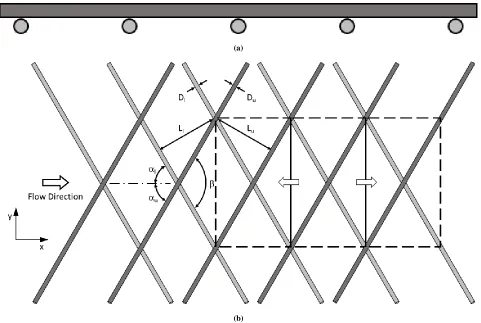
Fig. 2. Conventional non-woven symmetric diamond spacers: a) side view along lower filament and b) top view. The darker filaments are the upper filaments. The critical dimensions are: 1) filament diameter, Di; 2) spacing between filaments, Li; 3) angle between filament and flow direction, αi; and 4) angle between filaments, β, where the subscript i indicates the lower (l)

or upper (u) filaments. The dashed box indicates the unit cell used in the simulations for the symmetric spacer. Translating this unit cell in the x and y directions provides the velocity field at any point in a larger section of a symmetric spacer. The arrows indicate such a translation one unit cell width left and right in the x direction.

2. Methods

In this work, theoretical velocity profiles in spacer-filled channels are reported from CFD simulations and compared to experimental measurements obtained using PIV. CFD simulations were performed in COMSOL Multiphysics using a finite element based numerical approximation to the governing conservation of the momentum and mass equations. 2D-PIV studies were performed for conventional spacers and stereoscopic PIV studies were conducted for a novel static mixing spacer.

2.1. Spacers and test cells

The symmetric diamond spacer used in this work is illustrated in Figure 3. It consists of two overlapping filaments of equal diameter (0.254 mm) with an inter-filament angle of 60°. Figure 3 also illustrates the experimental test cell constructed by sandwiching a 45 mm × 50 mm x 0.5 mm sheet of the spacer between two microscope slides of dimensions 50 mm × 75 mm. Two needles provided a means to introduce and remove fluid. The needles and spacer were aligned such that the flow attack angle, the angle between the primary flow direction and the filaments, was 30o_{. Cell edges were sealed with epoxy.}

(a) (b)

(a) (b)

Fig. 4. Asymmetric spacer: a) experimental flow cell and b) domain used for simulations.

The asymmetric spacer used in this work is illustrated in Figure 4. It consists of a smaller filament (0.419 mm) overlapping a larger filament diameter (0.343 mm) at a 45°. The test cell for the spacer also in illustrated in

Figure 4 and is similar to that used for the symmetric spacer. The geometric

parameters for the symmetric and asymmetric spacers are summarized in

Table 1.

Novel static mixing spacers (Figure 5) were introduced by Iranshahi et al.

[25,26] to improve mass transfer in membrane modules. The spacers function

like the static mixers used in pipes with one exception: the fluid adjacent to the channel wall in the planar mixer is moved from the wall to the middle of the flow channel unlike the pipe equivalent. The longitudinally repeating section of the spacer is shown in Figure 5b. The front lip of the spacer divides the approaching fluid into two parts. The fluid above the lip is forced to flow into one of the openings along the length of the spacer as illustrated in Figure 5b and 5c. These openings (down-flow chimneys) provide a path from the upper part of the flow channel to the lower. Laminar flow of the fluid through the opening results in fluid adjacent to the upper membrane moving to the center of the flow channel and fluid from the middle of the flow channel flowing down to contact the lower membrane. Similar fluid movement occurs for the fluid below the lip: fluid is forced into an up-flow chimney through which it moves from the lower part of the channel to the upper. The induced movement of fluid streamlines from the membrane surface to the center of the flow channel is illustrated in Figure 5e.

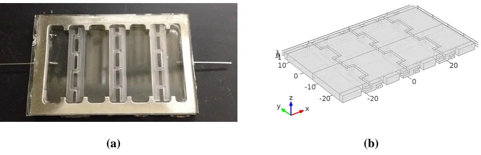
The flow pattern depends on several geometric parameters for the configuration shown: depth of chimney (A), width of chimney (B), length of front and rear lips (C), and thickness of chimney and lip structures (D). The values of the parameters for the spacer used are provided in Table 2. Figure 6 shows the arrangement of three static mixing spacer elements of 40 mm length separated by 10 mm. The spacers were held in a metallic frame that was sandwiched between two microscopic slides of 50 mm × 75 mm. Holes of 0.8 mm diameter were drilled to serve as inlet and an outlet. The edges of the test cell were sealed with epoxy.

2.2. 2D flow-visualization

Particle Image Velocimetry (PIV) is used for non-intrusive qualitative and quantitative velocity field measurements. Figure 7 illustrates the 2D-PIV experimental set-up [27]. In 2D-PIV, light is passed through the flow-cell and a set of successive images of moving particles is captured with a prescribed short time interval between images. The 2D-PIV experimental set-up consists of the flow-cell, a syringe pump to circulate the tracer suspension through the cell, a light source to illuminate the particles, a microscope with camera to view, focus and capture images of moving tracer particles, a timer to synchronize operation of the light source and camera, and data acquisition and analysis software. A suspension of tracer particles was prepared using 1 ml of 2% tracer solution and 50 ml of de-ionized water. FluoSpheresTM

carboxylate-modified Nile-Red microspheres (Life Technologies Corporation) was used as the tracer. A programmable syringe pump (KD Scientific) was used to pump the liquid at a specified flow rate. The actual flow rate was verified by measuring the flow-rate at the outlet through timed collection of a prescribed volume.

A Prior ProScan II translation stage was used to change the x-y position of focus. The flow cell was aligned normal to the gravitational field on the stage. A level was used to verify the horizontal arrangement. Due to the uneven edges created by the epoxy seal, some deviation from level is expected between the upper and lower planes of the flow cell but the deviation was measured to be less than ±5˚. An Olympus X741 microscope with a 10x lens was focused on an x-y plane at the desired z-position. Dantec Dynamics Studio v4 was used to acquire and analyze PIV data. Calibration of the experimental set-up required determination of the scale factor: mm distance per image pixel. The scale factor was determined using a rectangular rod of known 0.5 mm width. The camera and lens were adjusted to view the central region of the flow-cell. A double-pulsed laser light source was triggered by the PIV software program. The time-interval was selected such that particle displacement during the time-interval was sufficient to permit accurate displacement without the particles moving out of the interrogation area. About 30 pairs of images were captured at 6.1 Hz. Adaptive correlation was used to obtain spatial velocity maps from the images.

The spatial resolution of PIV is governed by the CCD sensor resolution of the camera and the magnification of the microscope used to obtain images. The camera possessed a 1344×1024 sensor array and with the microscope magnification a spatial resolution of 4.75 micron per pixel was achieved. For image analysis using adaptive correlation, each image was divided into subarea of 32×32 pixels with 25% overlap. The imaged region was approximately 1.5 mm in diameter.

Velocity vectors were obtained in three planes normal to the z-axis of the flow cell (parallel to the top and bottom surfaces) that pass through: 1) the center of the lower set of filaments, 2) the contact point between the upper and lower filaments, and 3) the center of the upper set of filaments. Table 3 summarizes parameters associated with the 2D-PIV system.

Table 1

Symmetric and asymmetric spacer geometric design parameters.

Spacer Dl (mm)

Du

(mm) Ll

(mm) Lu

(mm) αl

(°) αu

(°) β (°) Symmetric 0.25 0.25 1.64 1.64 30 30 60 Asymmetric 0.419 0.343 3.63 2.54 0 45 45

Table 2

Static mixing spacer geometric design parameters.

(a) (b)

(c)

(e)

Fig. 5. Static mixing spacer geometry: a) section of spacer with dashed box around repeat unit; b) three-dimensional view of repeat unit of spacer; c) top view of spacer with design dimensions and dashed box around repeat unit; d) side view of spacer with design dimensions. Spacer lies in x-y plane and arrows indicate flow direction (x-direction); and (e) fluid streamlines in static mixing spacer [25, 26].

(a)

(b)

Table 3

2D-PIV system parameters for symmetric and asymmetric spacers.

Parameter Symmetric Asymmetric

Cell dimension 50 mm × 75 mm x 0.5 mm 50 mm × 75 mm × 0.762 mm Spacer dimension 45 mm × 50 mm × 0.5 mm 45 mm × 50 mm × 0.762 mm Time between pulse 2000 - 3500 s 8000 - 12000 s

Scale factor 0.21

Acquisition mode Double frame mode

Seeding particles FluoSpheresTM _{carboxylate – modified microspheres, Nile-Red density – 1.033 g/cc}

Average diameter 1 m Particle concentration 1:50 v/v

Light source Double-pulse Nd:YAG Laser Wavelength 1064 nm, 532 nm Pulse duration 300 ns

Camera CCD HiSense Mk II camera Number of images 30

Trigger rate 6.1 Hz Interrogation area 32 × 32 pixels

Fig. 7. Schematic of experimental set up for 2D PIV.

2.3. Stereoscopic 3D flow visualization

Stereoscopic PIV requires two cameras aligned at a prescribed angle to each other to capture in-and-out of plane particle movement in the region of interrogation. A Scheimpflug condition is established such that the object, image, and lens planes intersect each other on the same line as illustrated in

Figure 8 [27]. Two manual focus Nikon telephoto Micro-Nikkon 105mm

f/2.8 AIS cameras and a Dantec Dynamics micro-strobe 9080X6901 were used to perform the experiments. The set-up was calibrated using a pin-hole calibration method. After calibration, the flow cell was placed such that the camera could be focused in the central region of the cell using a translation stage (Thorlabs MT1- 1/2”) without disturbing the position of each camera. A tracer solution was pumped through the cell at rate of 0.25 ml/min and particles in a plane of finite thickness were illuminated by the micro-strobe. Approximately 40 images of moving particles were captured by each camera

at a frequency of 10 Hz and stored in an image database for analysis. Velocity vectors were obtained through image processing using a combination of adaptive correlation and vector statistics. The software provided a 2D velocity vector map of in-plane velocity components and a scalar map of the out-of-plane velocity component.

The Reynolds number for the symmetric and asymmetric spacer is given by Equation Error! Reference source not found.:

(1)

using Equation Error! Reference source not found.[28]:

Fig. 8. Schematic of Scheimpflug condition for stereoscopic PIV [27].

(2)

where Hsp is flow channel height and  void fraction calculated using Equation

Error! Reference source not found.:

(3)

where Vsp is the volume of the spacer filament and Vtot total volume of the

flow channel. Ssp is the specific surface area of the spacer and calculated using

Equation Error! Reference source not found.:

(4)

where Dl is the diameter of the lower spacer filament and Du is the diameter

of the upper spacer filament. The Reynolds number for the static mixing spacer was calculated in a similar manner using the channel height for Dh

instead of Equation (2).

3. CFD Simulations

Laminar flow simulations were conducted for water at 21 °C using COMSOL Multiphysics. The conservation of mass equation (continuity equation) and conservation of momentum equations (Navier-Stokes equations) given by Equations (5) and (6), respectively:

ρ∇∙u=0 (5)

ρ(u∙∇u)=∇∙[-pI+μ(∇u+(∇u)T _{)]+F (6)}

were solved to obtain the pressure and velocity fields where ρ is the density of water, u velocity vector, p pressure, μ viscosity of water, and F volumetric force (i.e., gravity).

Solutions were obtained using meshes refined near solid boundaries to resolve the fine details of the flow field. For each spacer, a series of solutions were sought using progressively finer meshes to evaluate mesh sensitivity. The solution used for comparison to experiment differed by less than 10% on average between the two finest meshes used. The finest meshes contained up to four million mesh elements.

Flow domains representative of the spacer-filled flow cells were created in COMSOL Multiphysics. For simulations of the symmetric spacer, the unit cell identified in Figure 2 was used. The use of a unit cell to represent an infinite section of a spacer sheet is well documented in the literature [6, 20]. The unit cell is indicated by the central dashed box in Figure 2. The solution for the velocity field at any point in the spacer can be obtained by solving for the velocity field in the unit cell with periodic boundary conditions imposed on the top and bottom boundary pair (the two planes normal to the y direction) as the left and right boundary pair (the two planes normal to the x

direction). Due to the periodic nature of these boundaries, the unit cell can be translated left or right and up or down to obtain the velocity field at any other point. Figure 2 illustrates the translation of the unit cell to the left and right. The velocity field within the translated unit cells is identical to the velocity in the original unit cell. The velocity at any other point can be obtained through a similar set of translations.

Figure 3b illustrates the specific unit cell used. The filaments in the cell

overlapped with each other and the bounding surfaces by 25 µm. This overlap eliminates the sharp boundaries that would exist with point contact and are difficult to resolve in the simulations. Additionally, it reflects the geometry of real spacers with greater fidelity. The flow domain has a height of 0.425 mm (2x diameter minus 3x overlap) which is nearly identical to that of the experimental flow cell.

Boundary conditions for simulations of the unit cell flow domain for the symmetric spacer are:

1. In and out-flow bounding planes (planes normal to the x direction) – periodic boundary condition

The velocities along each boundary are identical: uin-flow = uout-flow. The

pressure along the boundaries differs by a prescribed amount (p) which is used to set the flow rate: pin-flow = pout-flow+p.

2. Left and right lateral bounding planes (planes normal to the y direction) – periodic boundary condition

The velocities and pressure along each boundary are identical: uleft = uright

and pleft = pright.

3. Top and bottom bounding surfaces (planes normal to the z direction) and filament surfaces – no slip boundary condition.

The velocity is set equal to zero: u = 0.

For simulations of the asymmetric spacers, the entire flow-cell used experimentally was created and meshed in COMSOL for the simulations as an appropriate repeating unit-cell is not obvious. Similarly, the entire flow-cell was created and meshed in COMSOL for the static mixing spacer, as each static mixing spacer element had only three repeating unit-cells. Figures 4b and 6b illustrate the simulation domains for the asymmetric and static mixing spacers, respectively.

Boundary conditions for simulations of the full flow domain for the asymmetric and static mixing spacer are:

1. Along the inlet opening– fixed, uniform velocity The velocity is set to a uniform value: uinlet=ufixed.

2. Along the outlet opening – outflow boundary and atmospheric pressure The pressure is set to atmospheric at a point along the outlet boundary poutlet=patmospheric.

3. All other boundary surfaces and filament surfaces – no slip boundary condition.

The velocity is set equal to zero: u = 0.

4. Results and discussion

Two-dimensional experimental measurements and simulation values are compared for the symmetric and asymmetric spacer. Qualitative and quantitative comparisons are provided. Three-dimensional comparisons are provided for the static mixing spacer which has the greatest out of plane velocities.

4.1. Symmetric spacer

Results are presented for the three x-y planes illustrated in Figure 9: (1) bottom – through the center of the bottom filaments, (2) middle – through the contact line between the bottom and top filaments, and (3) top – through the center of the top filaments-plane. Velocity magnitudes along the vertical and horizontal lines illustrated in Figure 10 within each the three planes are compared.

Figure 11 qualitatively compares the experimental vector velocity field to

simulation results in the bottom plane. The filaments in this plane run from the lower left-corner of Figure 11 to the upper right corner. The velocity field in the central region between the filaments is primarily in the nominal flow direction (x direction) from left to right. The flow is parallel to the lower set of filaments (perpendicular to the upper set of filaments) in the lower left and upper right corners where it passes under the upper set of filaments.

Figures 12 and 13 quantitatively compare the x and y velocity

in the nominal flow direction (x direction). Along the vertical line, both velocity components increase from the beginning of the line, pass through an apparent maximum and then decrease at the end. The decrease at the ends of the line arises from the proximity of the stationary filament along which the fluid velocity is identically zero. The changes in the x velocity are greater than the y velocity because this is the nominal flow direction (x direction). Additionally, the maximum x velocity is approximately equal to the value along the horizontal line as expected.

(a)

(b)

(c)

Fig. 9. Planes imaged within symmetric and asymmetric spacer: a) top plane through center of the top filaments, b) middle plane through contact line between filaments, and c) bottom plane through center of bottom filaments (closest to camera).

Fig. 10. Horizontal and vertical lines for quantitative velocity comparisons within symmetric spacer. The arrow heads indicate the direction along which the coordinate increases.

The greatest quantitative differences in velocity exist for the x component at the end of the vertical line. These differences most likely are due to deviations between the experimental and simulated spacer geometry (such as deviations from a uniform cylindrical shape and uniform angle between filaments), how precisely the interrogation plane can be selected in the experiments (small deviations from the center of the filament will change the dimensions of the fluid filled area especially near the filaments), and the difficulty of obtaining velocities near filaments where rapid changes in velocity occur. Figure 14 illustrates the experimental vector velocity field in the bottom plane near the point of contact between the lower and upper filaments. The rapid change in velocity near the lower filament, extending left bottom to right top, is evident which limits the ability to resolve velocity in this region. Qualitative and quantitative results for the top plane are nearly identical.

Figures 15 and 16 quantitatively compare the x and y velocity

components in the middle plane, through the filament contact line, along the horizontal and vertical lines in Figure 10, respectively. Qualitative comparisons of the experimental and simulated vector velocity fields are

similar to Figure 11. As found for the bottom plane, quantitative agreement is good. The maximum x velocities are greater in the middle plane than the bottom or top planes because the filaments force fluid from both the upper and lower halves of the flow channel to the middle to pass around the filaments. The greatest quantitative deviations are found at the end of the vertical line and attributed to the same factors as for the bottom plane.

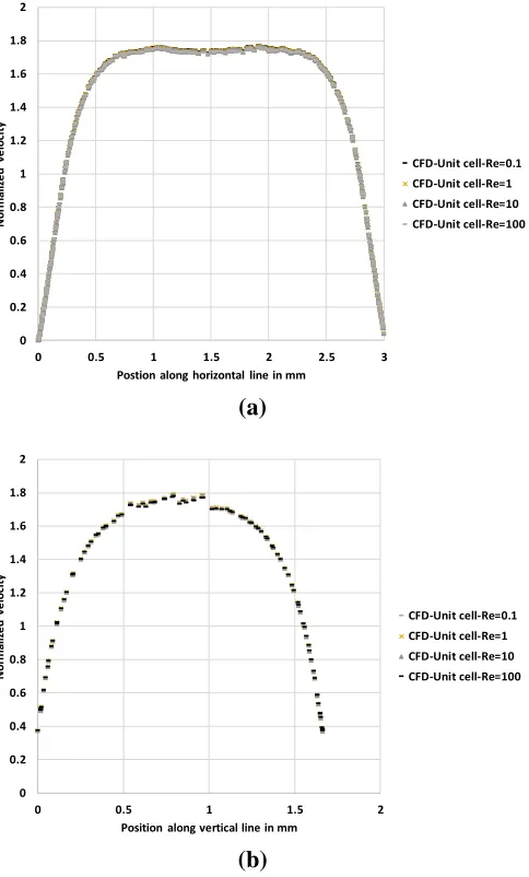
The experimental results presented here are for Reynolds numbers less than 1. To demonstrate the results are valid for higher Reynolds numbers encountered in application, simulations were conducted using the unit cell illustrated in Figure 3 for Reynolds numbers up to 100. The simulations were performed using the same boundary conditions as described previously but with large pressure drops across the unit cell to increase the Reynolds number. Mesh refinement and convergence conditions also were identical. The x-component of velocity in the middle plane along the horizontal and vertical lines in Figure 10 is illustrated in Figure 17. The values are normalized with the superficial velocity, i.e., volumetric flow rate divided by channel cross-sectional area. Changes in the normalized velocity with Reynolds number are not discernable indicating the results at low Reynolds are representative of results throughout the laminar flow regime.

An additional difference between experiment and simulation is the simulation assumes a well-developed flow within a large section of the spacer (represented by the unit cell in Figure 3) while the experiment utilizes a flow cell with a single inlet and outlet containing a finite spacer section. To evaluate the effect of cell finiteness and inlet/outlet port location, simulations were performed for the experimental conditions using the exact geometry of the flow cell. The simulations utilized no-slip boundary conditions along all surfaces of the unit cell except for the inlet and outlet boundaries which were treated as a uniform in-flow and out-flow, respectively. Figure 18 illustrates the velocity field within the middle plane of the flow cell. The flow from the inlet port quickly rearranges to a uniform flow before entering the spacer section. The values for x and y velocity components along the horizontal and vertical lines in Figure 10 also are illustrated in Figures 15 and 16, respectively. The results for the unit cell and the full flow cell vary by less than 10%. Similar results are observed in the bottom plane as illustrated in

Figures 12 and 13. Such agreement indicates the unit cell provides a good

representation of the experimental results.

To assess the experimental error associated with the reported PIV velocities, experiments were performed for flow rates ranging from 0.25 to 0.75 ml/min. The results are shown in Figure 19 for the variation of the x component of the velocity along the horizontal and vertical lines in Figure 10. The velocity values are normalized by the superficial velocity to permit comparison. The differences in the normalized velocities are less than 10% indicating the experimental error.

4.2. Asymmetric spacer

Results are presented for the same three x-y planes illustrated in Figure 9. However, experimental and simulated velocity magnitudes are compared along the vertical and horizontal lines illustrated in Figure 20. Only quantitative comparisons are provided as qualitative results are similar to

Figure 11.

Figures 21 and 22 provide a quantitative comparison of x and y velocity

components in the top plane along the horizontal and vertical lines in Figure 20, respectively. The smaller filaments that are at 45° to nominal flow direction (x direction) lie in this plane. Good agreement exists between experiment and simulation. Figure 21 indicates the x velocity is nearly constant along the horizontal line indicating a uniform flow in the nominal flow direction (x direction). A y velocity exists that is induced by the upper filaments; this velocity component redistributes the flow across the width of the channel. Figure 22 indicates both velocity components increase along the vertical line as the distance from the filament increases. The velocity appears to approach a maximum but a decrease is not observed at the end of the vertical line as observed for the symmetric spacer in Figure 13. A decrease is not observed because the vertical line used to report the asymmetric spacer results extends only half-way between the two filaments while that used to report the symmetric spacer results ends much closer to the second filament.

Fig. 11. Vector velocity field in the bottom plane for a flow rate of 0.25 ml/min (Re = 0.1): a) PIV results and b) simulation.

-0.05 0 0.05 0.1 0.15 0.2 0.25 0.3 0.35

0 0.2 0.4 0.6 0.8 1 1.2 1.4

V

el

oci

ty

com

p

on

en

t i

n

m

m

/s

Position along horizontal line in mm

PIV-Ux CFD-Ux-Flow cell CFD-Ux-Unit cell PIV-Uy CFD-Uy-Flow cell CFD-Uy-Unit cell

Fig. 12. Velocity variation in the bottom plane along the horizontal line for the symmetric spacer at a flow rate of 0.25 ml/min (Re = 0.1).

-0.05 0 0.05 0.1 0.15 0.2 0.25 0.3 0.35

0 0.2 0.4 0.6 0.8 1 1.2

V

el

oci

ty

com

p

on

en

t i

n

m

m

/s

Position along horizontal line in mm

PIV-Ux CFD-Ux-Flow cell CFD-Ux-Unit cell PIV-Uy CFD-Uy-Flow cell CFD-Uy-Unit cell

Fig. 13. Velocity variation in the bottom plane along the vertical line for the symmetric spacer at a flow rate of 0.25 ml/min (Re = 0.1).

Fig. 14. Experimental vector velocity field near point of filament contact for symmetric spacer.

-0.05 0 0.05 0.1 0.15 0.2 0.25 0.3 0.35 0.4 0.45

0 0.2 0.4 0.6 0.8 1 1.2 1.4

V

el

oci

ty

com

p

on

en

t i

n

m

m

/s

Position along horizontal line in mm

PIV-Ux CFD-Ux-Flow cell CFD-Ux-Unit cell PIV-Uy CFD-Uy-Flow cell CFD-Uy-unit cell

-0.05 0 0.05 0.1 0.15 0.2 0.25 0.3 0.35 0.4 0.45

0 0.2 0.4 0.6 0.8 1 1.2

V el oci ty com p on en t i n m m /s

Position along horizontal line in mm

PIV-Ux CFD-Ux-Flow cell CFD-Ux-Unit cell PIV-Uy CFD-Uy-Flow cell CFD-Uy-Unit cell

Fig. 16. Velocity variation in the middle plane along the vertical line for the symmetric spacer at a flow rate of 0.25 ml/min (Re = 0.1).

0 0.2 0.4 0.6 0.8 1 1.2 1.4 1.6 1.8 2

0 0.5 1 1.5 2 2.5 3

N o rm al iz e d V e lo ci ty

Postion along horizontal line in mm

CFD-Unit cell-Re=0.1 CFD-Unit cell-Re=1 CFD-Unit cell-Re=10 CFD-Unit cell-Re=100

(a)

0 0.5 1 1.5 2

N o rm al iz e d ve lo ci ty

Position along vertical line in mm

CFD-Unit cell-Re=0.1 CFD-Unit cell-Re=1 CFD-Unit cell-Re=10 CFD-Unit cell-Re=100

(b)

Fig. 17. Normalized velocity in middle plane of unit cell of symmetric spacer at Re = 0.1, 1, 10, and 100: a) along horizontal line illustrated in Figure 10 and b) along vertical line illustrated in Figure 10.

Fig. 18. Velocity profile (normalized to average velocity in flow cell) in middle plane from simulation in flow cell of symmetric spacer with single-needle point inlet and outlet.

0 0.5 1 1.5 2 2.5

0 0.2 0.4 0.6 0.8 1 1.2 1.4

N o rm al iz e d ve lo ci ty

Postion along horizontal line in mm

CFD-Flowcell-0.25ml/min CFD-Flowcell-0.5ml/min CFD-Flowcell-0.75ml/min PIV-Flowcell-0.25ml/min PIV-Flowcell-0.5ml/min PIV-Flowcell-0.75ml/min

(a)

0 0.2 0.4 0.6 0.8 1 1.2 1.4

N o rm al iz e d ve lo ci ty

Position along vertical line in mm

CFD-Flowcell-0.25ml/min CFD-Flowcell-0.5ml/min CFD-Flowcell-0.75ml/min PIV-Flowcell-0.25ml/min PIV-Flowcell-0.5ml/min PIV-Flowcell-0.75ml/min

(b)

Fig. 20. Horizontal and vertical lines for quantitative velocity comparisons within asymmetric spacer. The arrow heads indicate the direction along which the coordinate increases.

0 0.05 0.1 0.15 0.2 0.25

0 0.2 0.4 0.6 0.8 1 1.2 1.4

V

e

loc

ity

comp

on

e

n

t

in

mm/

s

Position along horizontal line in mm

PIV-Ux CFD-Ux PIV-Uy CFD-Uy

Fig. 21. Velocity variation in the top plane along the horizontal line for the asymmetric spacer at a flow rate of 0.25 ml/min (Re = 0.1).

0 0.05 0.1 0.15 0.2 0.25 0.3

0 0.2 0.4 0.6 0.8 1 1.2

V

e

loc

ity

comp

on

e

n

t

in

mm/

s

Position along horizontal line in mm

PIV-Ux CFD-Ux PIV-Uy CFD-Uy

Fig. 22. Velocity variation in the top plane along the vertical line for the asymmetric spacer at a flow rate of 0.25 ml/min (Re = 0.1).

4.3. Static mixing spacer

Results are presented for the section of the spacer illustrated in Figure 5b. This section of the spacer includes the fluid flow region in front of the leading edge of the spacer and one of the chimneys through which fluid flows through the spacer. The selected chimney is a down flow chimney that directs flow from the upper half of the flow channel to the lower half.

Figure 23 illustrates the experimental x-y vector velocity field

superimposed on a color mapping of the z velocity component for a plane that passes along the top edge of the spacer. The region in the figure without velocity data (velocity vectors or color map), corresponds to the leading edge that divides the flow. The yellow-red color coding indicates z velocities coming out of the plane towards the reader while blue indicates velocities going into the plane. The blue area occupies a rectangular region corresponding to the down flow chimney where fluid flows from the upper part of the flow channel to the lower part. Because the leading edge of the spacer possesses a finite thickness, it will force a portion of the fluid flow upward into the upper half of the flow channel and a portion downward into the lower half. The yellow-red area corresponds to the region where fluid is forced upwards. The largest downward velocities are approximately three times greater than the largest upward velocities. This is consistent with the observation that the flow through the chimney is equal to the flow through half of the flow channel height while the upward flow induced by the leading edge corresponds to the flow through roughly half of the thickness of the leading edge – the ratio of one-half the flow channel height to one-half the leading edge thickness (or equivalently the ratio of the flow channel height to the leading edge thickness) is approximately 3 based on the geometry in

Figure 5.

Fig. 23. Experimental x-y vector velocity field superimposed on color mapping of z velocity. Green indicates a value of zero velocity and the green area corresponds to the location of the spacer. The dashed black lines indicates the leading lip of the spacer and lip edges in the chimneys. The solid black line indicates the chimney boundary. The white line indicates the location of the quantitative velocity comparisons in Figure 24. The arrow indicates the direction of increasing coordinate value.

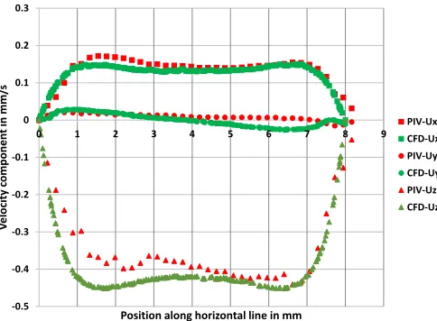
Figure 24 compares the experimental and simulated values of the three

velocity components along the line in the down flow chimney indicated in

Figure 23. Excellent agreement is observed for all three components. The z

-0.5 -0.4 -0.3 -0.2 -0.1 0 0.1 0.2 0.3

0 1 2 3 4 5 6 7 8 9

V

e

loc

ity

comp

on

e

n

t

in

mm/

s

Position along horizontal line in mm

PIV-Ux CFD-Ux PIV-Uy CFD-Uy PIV-Uz CFD-Uz

Fig. 24. Velocity variation along the line in Figure 23 located within the down flow chimney for the static mixing spacer at a flow rate of 1 ml/min (Re = 0.52).

5. Conclusions

Simulations of flow in spacer filled channels are compared to experimental measurements using particle image velocimetry. Comparisons of the simulated and experimental in-plane 2D velocity components are in good agreement. The flow in-between filaments is primarily in the nominal flow direction (x direction) with rapid changes near the filaments where fluid velocity is zero and fluid is forced around filaments. The largest changes occur near the point where filaments are in contact.

3D velocity measurements for a static mixing spacer also are reported. All three fluid velocity components show good agreement between simulated and experimental values. The experiments confirm the ability to simulate flow through the chimneys of the spacer as required to move fluid from adjacent to the membrane surface to the middle of the flow channel. This movement can help reduce concentration polarization.

The results provide support for the use of computational fluid mechanics to predict the components of the velocity field within spacer filled channels. A full comparison of all three velocity components is presented in contrast to past work. Such an ability is required to perform simulations of mass transfer and ultimately seek to optimize spacer design.

Acknowledgements

This work was performed as part of a research program supported the U.S. Department of Energy Project No. DE-FE0007553.

References

[1] J. Johnson, M. Busch, Engineering Aspects of Reverse Osmosis Module Design, Desal. Water Treat. 15 (2010) 236-248.

[2] J. Schwinge, D.E. Wiley, D.F. Fletcher, Simulation of the Flow around Spacer Filaments between Narrow Channel Walls. 1. Hydrodynamics, Ind. Eng. Chem. Res. 41 (2002) 2977-2987.

[3] A. Saeed, R. Vuthaluru, Y. Yang, H.B. Vuthaluru, Effect of feed spacer arrangement on flow dynamics through spacer filled membranes, Desalination 285 (2012) 163-169.

[4] G.A. Fimbres-Weihs, D.E. Wiley, Review of 3D CFD modeling of flow and mass transfer in narrow spacer-filled channels in membrane modules, Chem. Eng. Process. 49 (2010) 759-781.

[5] P. Willems, N.G. Deen, A.J.B. Kemperman, R.G.H. Lammertink, M. Wessling, M. van Sint Annaland, J.A.M. Kuipers, W.G.J. van der Meer, Use of Particle Imaging Velocimetry to measure liquid velocity profiles in liquid and liquid/gas flows through spacer filled channels, J. Membr. Sci. 362 (2010) 143-153.

[6] C.P. Koutsou, S.G. Yiantsios, A.J. Karabelas, Direct numerical simulation of flow in spacer-filled channels: Effect of spacer geometrical characteristics, J. Membr. Sci. 291 (2007) 53-69.

[7] O. Kavianipour, G.D. Ingram, H.B. Vuthaluru, Investigation into the effectiveness of feed spacer configurations for reverse osmosis membrane modules using Computational Fluid Dynamics, J. Membr. Sci. 526 (2017) 156-171.

[8] K. In Seok, C. Ho Nam, The effect of turbulence promoters on mass transfer— numerical analysis and flow visualization, Int. J. Heat Mass Tran. 25 (1982)

1167-1181.

[9] W.S. Kim, J.K. Park, H.N. Chang, Mass transfer in a three-dimensional net-type turbulence promoter, Int. J. Heat Mass Tran. 30 (1987) 1183-1192.

[10]A.R. Da Costa, A.G. Fane, D.E. Wiley, Spacer characterization and pressure drop modeling in spacer-filled channels for ultrafiltration, J. Membr. Sci. 87 (1994) 79-98.

[11]C.C. Zimmerer, V. Kottke, Effects of spacer geometry on pressure drop, mass transfer, mixing behavior, and residence time distribution, Desalination 104 (1996) 129-134.

[12]S.K. Karode, A. Kumar, Flow visualization through spacer filled channels by computational fluid dynamics I. Pressure drop and shear rate calculations for flat sheet geometry, J. Membr. Sci. 193 (2001) 69-84.

[13]Z. Cao, D.E. Wiley, A.G. Fane, CFD simulations of net-type turbulence promoters in a narrow channel, J. Membr. Sci. 185 (2001) 157-176.

[14]P.R. Neal, H. Li, A.G. Fane, D. Wiley, The effect of filament orientation on critical flux and particle deposition in spacer-filled channels, J. Membr. Sci. 214 (2003) 165-178.

[15]M. Gimmelshtein, R. Semiat, Investigation of flow next to membrane walls, J. Membr. Sci. 264 (2005) 137-150.

[16]M. Shakaib, S.M.F. Hasani, M. Mahmood, Study on the effects of spacer geometry in membrane feed channels using three-dimensional computational flow modeling, J. Membr. Sci. 297 (2007) 74-89.

[17]Y. Gao, S. Haavisto, C.Y. Tang, J. Salmela, W. Li, Characterization of fluid dynamics in spacer-filled channels for membrane filtration using Doppler optical coherence tomography, J. Membr. Sci. 448 (2013) 198-208.

[18]T. Wang, Z. Zhang, X. Ren, L. Qin, D. Zheng, J. Li, Direct observation of single- and two-phase flows in spacer filled membrane modules, Sep. Purif. Technol. 125 (2014) 275-283.

[19]S.M. Mojab, A. Pollard, J.G. Pharoah, S.B. Beale, E.S. Hanff, Unsteady Laminar to Turbulent Flow in a Spacer-Filled Channel, Flow Turbul. Combust. 92 (2014) 563-577.

[20]Y. Lou, R. Gogar, P. Hao, G. Lipscomb, K. Amo, J. Kniep, Simulation of net spacers in membrane modules for carbon dioxide capture, Sep. Sci. Technol. 52 (2017) 168-185.

[21]A.H. Haidari, S.G.J. Heijman, W.G.J. van der Meer, Visualization of hydraulic conditions inside the feed channel of Reverse Osmosis: A practical comparison of velocity between empty and spacer-filled channel, Water Res. 106 (2016) 232-241. [22]A.H. Haidari, S.G.J. Heijman, W.G.J. van der Meer, Effect of spacer configuration

on hydraulic conditions using PIV, Sep. Purif. Technol. 199 (2018) 9-19. [23]S.S. Bucs, R. Valladares Linares, J.O. Marston, A.I. Radu, J.S. Vrouwenvelder, C.

Picioreanu, Experimental and numerical characterization of the water flow in spacer-filled channels of spiral-wound membranes, Water Res. 87 (2015) 299-310. [24]R.L. Gogar, Flow Investigation in Spacers of Membrane Modules, 2015, University

of Toledo.

[25]A. Iranshahi, Static Mixing Spacers for Spiral Wound Modules, 2012, University of Toledo.

[26]J. Liu, A. Iranshahi, Y. Lou, G. Lipscomb, Static mixing spacers for spiral wound modules, J. Membr. Sci. 442 (2013) 140-148.

[27]M. Raffel, C.E. Willert, S.T. Wereley, J. Kompenhans, Particle Image Velocimetry: A Practical Guide, 2nd _{Ed., Springer-Verlag, Berlin Heidelberg, 2007.}