https://doi.org/10.5194/esurf-7-247-2019 © Author(s) 2019. This work is distributed under the Creative Commons Attribution 4.0 License.
Modelling braided river morphodynamics using a particle
travel length framework
Alan Kasprak1,a, James Brasington2, Konrad Hafen1,3, Richard D. Williams4, and Joseph M. Wheaton1
1Department of Watershed Sciences, Utah State University, Logan, Utah 84322, USA
2Te Waiora, Institute for Freshwater Management, University of Waikato, Hamilton 3240, New Zealand 3Water Resources Program, University of Idaho, Moscow, Idaho 83844, USA
4School of Geographical and Earth Sciences, University of Glasgow, Glasgow, G12 8QQ, UK
anow at: US Geological Survey, Southwest Biological Science Center, Grand Canyon Monitoring and Research
Center, Flagstaff, Arizona 86001, USA
Correspondence:Alan Kasprak ([email protected])
Received: 13 February 2018 – Discussion started: 13 April 2018
Revised: 20 December 2018 – Accepted: 4 January 2019 – Published: 14 March 2019
1 Introduction
The dearth of morphodynamic models that resolve the bar-scale morphology of braided, gravel-bed rivers remains a first-order weakness in fluvial geomorphology. Indeed, since prediction is generally perceived to be the pinnacle of sci-entific enquiry, the limitations associated with existing mod-elling frameworks that can be used to inform management and natural hazard assessment of braided rivers restrict the contribution that our science can make to addressing so-cietal needs (Wilcock and Iverson, 2003). Focusing model development on braided rivers is paramount since, in prin-ciple, if a numerical framework can predict the evolution of multiple channels and bars during high-flow events in these multi-thread rivers, then the same framework should be transferable to single-thread rivers. Major progress has been made in applying contemporary measurement technolo-gies to quantify the morphodynamics of braided rivers at the timescale of individual to sequences of high-flow events (10−2–100 years; Lane et al., 2003; Wheaton et al., 2013; Williams et al., 2011, 2015; Lallias-Tacon et al., 2014). Prediction is, however, needed at the mesoscale (broadly 100–102km and 101–103 years; Brasington and Richards, 2007), which exceeds the scale of feasible field-based mon-itoring campaigns. There have been considerable advances in modelling realistic bar-scale morphology of fine-grained braided rivers at the mesoscale (Nicholas, 2013a; Schuurman et al., 2013; Schuurman, 2015) but models that resolve bar-scale morphology of gravel-bed rivers at timebar-scales greater than single high-flow events (Williams et al., 2016b) remain challenging. Furthermore, while “physics-based” (Nicholas, 2013b) approaches to simulation have been successful for fine-grained rivers, such approaches have high computational overheads necessitating the use of high performance comput-ing resources and restrictcomput-ing their use for exploratory appli-cations (e.g. Nicholas, 2013a). The additional computational demand of simulating sediment mixtures, combined with the extant problems of spatial parameterization of sediment char-acter, limits the scope of comparable “physics-based” ap-proaches to gravel-bed river simulations. There is, therefore, a need to develop an alternative computationally efficient morphological modelling framework capable of reproduc-ing realistic bar-scale morphodynamics of braided gravel-bed rivers over geomorphologically meaningful timescales (101–103years).
A variety of spatially distributed morphodynamic mod-elling frameworks have been developed to address this prob-lem and are reviewed in depth by Williams et al. (2016a). Current approaches have been broadly assigned into one of two philosophical categories. The first involves simplifying and abstracting physical processes using a set of rules or sim-plified algorithms, giving rise to so-called “reduced complex-ity” (RC) models, often in the form of cellular automata (CA) models (RC/CA; Murray and Paola, 1994; Coulthard et al., 2002; Thomas and Nicholas, 2002). These rule-based
mod-els offer high computational efficiency, allowing calculations over wide spatial and long temporal scales (e.g. Nicholas and Quine, 2007; Thomas et al., 2007; Ziliani et al., 2013), but often at the expense of morphological fidelity to any par-ticular system, instead producing self-organization and gen-eralized behaviours of a given channel type (e.g. Murray and Paola, 1994; Murray, 2003). RC/CA models are partic-ularly well suited for investigating the generalized morpho-dynamic response of channels under shifting boundary con-ditions (Thomas et al., 2007). The alternative second sub-set of models is widely referred to as physics-based, and are driven by computational fluid dynamics schemes (CFD; Bates et al., 2005) typically involving two-dimensional ap-proximations of solutions to the Navier–Stokes equations. Bed shear stress is used as a measure of the friction force imposed by flow to scale bedload transport. The direction and distance of bedload transport are calculated based upon the flow field and parameterizations are employed to repre-sent gravity-driven sediment transport, particle settling and remobilization effects. The Exner equation (Paola and Voller, 2005) is then used to calculate bed elevation change from lo-cal sediment flux divergence. This physics-based approach to calculating morphodynamic evolution comes at the cost of significantly increased computational overheads, particu-larly for graded sediment. Nonetheless, physics-based mod-els have been widely applied to simulate fluvial systems (Mosselman et al., 2000; Rinaldi et al., 2008; Kleinhans, 2010) and event-based, graded sediment simulations repro-ducing reach-scale morphodynamics of natural rivers are be-ginning to emerge (Williams et al., 2016b). Moreover, such models have been used to shed light on how the morpho-dynamics of braided rivers are influenced by sediment het-erogeneity (Sun et al., 2015; Singh et al., 2017) and vegeta-tion (Crosato and Saleh, 2011; Li and Millar, 2011; Nicholas et al., 2013a; Iwasaki et al., 2017). Despite this progress, mesoscale physics-based simulations require considerable computational resources and can diverge from predicting fea-sible morphology (Schuurman et al., 2015). Beyond this clas-sic dichotomy, a third approach to morphodynamic simula-tion draws on particle-based methods from granular physics (Frey and Church, 2012). This approach is, however, compu-tationally intensive and the absence of appropriate upscaling methods limits its application to patch-scale investigations of sediment entrainment, transport, and deposition (e.g. Escau-riaza and Sotiropoulos, 2011; Nabi et al., 2013).
(evolution of the bed). Furthermore, an approach to sedi-ment transport modelling based on particle path lengths, the characteristic distance travelled by sediment particles dur-ing a flood (Davy and Lague, 2009; Furbish et al., 2016), has potential to simplify simulation of bedload transport rep-resenting the fundamental process that leads to bar forma-tion and morphodynamics. Recent work indicates that mor-phology, bed structure, and texture play a key role in par-ticle dispersion (Hassan and Bradley, 2017). Parpar-ticle path-length distributions have been found to take several forms in braided gravel-bed rivers, including exponential decay, or heavy-tailed distributions, marked by a large number of mo-bilized particles short distances downstream, resulting from floods that do not generate sufficient shear stress for transport across the braidplain width (Pyrce and Ashmore, 2003b). During floods which are capable of transporting sediment (i.e., competent) across large areas of the braidplain, typical path-length distributions exhibit peaks which correspond to the location of likely depositional sites downstream. Kasprak et al. (2015) and Pyrce and Ashmore (2003a, b) both noted that these depositional sites were most frequently the loca-tions of bar heads (e.g. flow diffluences); and as such, par-ticle path-length distributions could be readily constructed using morphometric indices that reflect the characteristic confluence–diffluence spacing.
This paper presents a new hybrid morphodynamic mod-elling approach that employs two-dimensional CFD hy-draulics resolved at the event scale and a rule set for sediment transport that leverages hydraulic predictions to determine particle path lengths along which to erode and route sediment and subsequently evolve topography. Previous research on particle path-length distributions has largely been conducted in braided gravel-bed rivers; and as such, the model described here, termed MoRPHED (Model of Riverine Physical Habi-tat and Ecogeomorphic Dynamics), has been developed for such environments. Characteristic particle travel distances have, however, also been documented for single-thread chan-nels (Pyrce and Ashmore, 2003b), so it may therefore be pos-sible to apply the underlying theory to a wide variety of chan-nel forms. That said, the approach is only appropriate where the extremes of the path-length distribution are less than the length of the system to be modelled (i.e. for gravel- rather than sand-bed rivers).
Combining both dynamical (force-based hydraulics) and kinematic (motion-based prediction of particle transport) frameworks provides an effective compromise that incorpo-rates the necessary physics to simulate the key driving forces and vectors of motion, but simultaneously offers a reduced complexity structure suitable for wide-area, long-term mor-phodynamic modelling. This paper explores the degree to which MoRPHED can (a) capture the emergent properties of natural fluvial environments; (b) maintain, but not neces-sarily form or produce, braided topography; and (c) exhibit sensitivity to contrasting process representations.
For transparency and ease of future development, the model presented here has been packaged into an open-source code published at https://github.com/morphed/MoRPHED (last access: 22 February 2019) and includes a user inter-face (https://github.com/morphed/MoRPHED-Viewer, last access: 22 February 2019). The novel contributions set out in this paper are (i) a new numerical morphodynamic mod-elling framework that combines a dynamics-based CFD ap-proach to predicting flow routing and a kinematics-based par-ticle travel length rule set for sediment transport and mor-phological change; (ii) testing the modelling framework us-ing data from two contrastus-ing natural rivers, with sensitiv-ity analyses to assess hydrograph discretization strategies and path-length statistical distributions; and (iii) multi-scalar model verification using a plurality of rigorous validation approaches including reach-scale quantitative morphological change budgets and the pattern of contribution of different braiding mechanisms.
2 The model
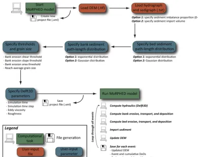
As with many previously developed morphodynamic mod-els, the model used here (MoRPHED v.1.1) simulates hy-draulics and uses these calculations to predict bedload trans-port and morphological change. This section details the methods used in each of these components, along with ancil-lary routines such as the parameterization of model bound-aries, sediment grain size, and bank erosion. Figure 1 shows a flow chart of model operation along with required and op-tional inputs and outputs; these components are discussed throughout this section.
2.1 Hydraulics
Figure 1.MoRPHED model operation flow chart.
ρ
u∂u ∂x+v
∂u ∂y
= −∂P ∂x +µ
∂2u ∂x2+
∂2u ∂y2
, (1)
ρ
u∂v ∂x+v
∂v ∂y
= −∂P ∂y +µ
∂2v ∂x2+
∂2v ∂y2
, (2)
wherexandy, respectively, denote the streamwise and cross-stream directions of velocity (u,v). In Eqs. (1)–(2), P de-notes pressure forces on a body of fluid,ρ is fluid density, andµdenotes dynamic viscosity. For all modelling, we em-ployed fixed Cartesian orthogonal grids which were gener-ated using the RGFGRID module of the Delft3D software suite. Elevation models used as Delft3D inputs were rotated such that flow was from left (upstream) to right (downstream) for use with a Cartesian coordinate system. The model time step was then adjusted to satisfy the Courant–Friedrichs– Levy condition to ensure computational stability of the so-lution.
For all simulations, discharge was specified at the up-stream boundary and a corresponding water surface eleva-tion was set to the downstream boundary, and was calculated using a normal depth approximation based on reach-average slope and roughness. Horizontal eddy viscosity (υ) was set to 0.1 s m−2(Williams et al., 2013). A spatially constant bed
roughness was used, based on the Colebrook–White equa-tion, to determine the 2-D Chezy coefficient:
C2-D=18log10
12H ks
, (3)
whereH is water depth andks is the Nikuradse roughness
length, which can be described in terms of a factor (αx) of
the characteristic grain diameter as
ks=αxD84. (4)
Here, we usedD84as the characteristic grain size as it
pro-vides an estimate of coarse grain influence on the flow field. Using grain size distributions available for both of the mod-elling sites in this paper (Hodge et al., 2009; Williams et al., 2013), we computedksusing anαxvalue of 2.9, taken as the
average value from a range of gravel-bed rivers studied in Garcia (2006). This resulted in values ofks=0.1 and 0.29 m
for the Rees River and River Feshie, respectively.
velocity resolved into streamwise and lateral components, and (c) bed shear stress. Put simply, flow hydraulics were computed for the maximum discharge of a given flood, and these hydraulics were used to drive subsequent sediment mo-bilization and morphodynamic evolution. This approach was adopted because (a) the calculation of morphodynamics once per event allows for a greatly reduced computational over-head associated with the model, and (b) modelling at finer timescales – while allowing for the ability to capture rapid transient events such as prograding bedload sheets and bank retreat during the course of a single flood – is inherently dif-ficult given that the most common observational data avail-able to geomorphologists describe channel form before and after a single event (Bertoldi et al., 2010; Williams et al., 2011; Mueller et al., 2014), and sediment transport distances, or path lengths, resulting from that event (Pyrce and Ash-more, 2003a, b; Snyder et al., 2009; Kasprak et al., 2015). We acknowledge that a single-flood time step may neces-sarily oversimplify morphodynamic evolution resulting from floods that are of sufficient duration to produce multiple en-trainment episodes for particles, or those floods that funda-mentally alter the bar spacing, and thus the path-length dis-tribution, for a reach of interest. While our motivation was to assess the validity of a purely event-based model time step, regardless of flood duration, we provide a nested exper-iment in which the hydrograph of a single flood event was schematized as a set of three steady discharges correspond-ing to the riscorrespond-ing limb, peak, and fallcorrespond-ing limb of the event (Sect. 4.2). This schematization was used in an attempt to evaluate (a) the model’s suitability for simulating floods of extended duration and (b) the need for quasi-dynamic flow predictions to capture distinct stage-specific morphodynamic processes, such as the dissection of bar-top chutes at falling stages (e.g. Wheaton et al., 2013).
2.2 Bed sediment erosion
The model employs a critical non-dimensional value of the bed shear stress (Shields stress) to determine whether sed-iment can be entrained at a particular location. The theory and threshold values of Shields stress for entrainment have been well studied in gravel-bed river settings. Incipient mo-tion for gravel occurs when the Shields stress (τ∗) exceeds 0.03–0.07 (Buffington and Montgomery, 1997; Snyder et al., 2009):
τ∗= τB
(ρs−ρ)gD
, (5)
whereρsis a characteristic sediment density (2650 kg m−3), g is acceleration due to gravity, and D is the median par-ticle size. The spatial distribution of local bed shear stress (τB) at steady flow was computed using Delft3D and the
critical Shields stress for sediment mobility was set to 0.05. The modelled bed shear varies significantly over small spa-tial regions (Wilcock et al., 2009) and could therefore lead to
large cell-to-cell variability in elevation change and unstable coupling of the bed topography and modelled hydraulics. To avoid such effects, the localτBwas computed by averaging
the 10 cells longitudinally upstream and downstream of the cell in question along streamlines derived from the Delft3D velocity vectors. Although lateral averaging of shear stress could additionally reinforce model stability, this was not ex-plored here. The result is a single average value of bed shear stress that is used for computation of scour depth at each cell. Most morphodynamic models compute bed elevation change using some form of the Exner equation for sediment continuity (Paola and Voller, 2005). In this equation, bed ele-vation (z) through time (t) is a function of the sediment sup-plied from upstream (Vs), the divergence of the sediment flux
through the reach boundaries (∇Qs) and the porosity of the
deposited sediment (γp).
∂z ∂t =
1 1−γp
∂V
s
∂t + ∇ ·Qs
(6)
To ensure computational stability, morphodynamics are typi-cally computed by solving Eq. (6) at fine time steps (seconds to minutes) using solutions from the equations of motion. However, MoRPHED is specifically designed to operate at the mesoscale; at model time steps equal to flood events (e.g. hours to days), the use of Eq. (6) would lead to the forma-tion of large depressions or mounds in the channel topogra-phy, and would drive subsequent computational instability. In short, an based model requires an analogous event-based approach for the estimation of bed elevation change. To drive the erosional component of bed elevation change (sediment transport and deposition are discussed in subse-quent sections), we used an alternative approach to the lo-cal sediment continuity equation, based on Montgomery et al. (1996) who derived a theoretical relationship to predict event-scale sediment scour depth (Ds):
Ds= Qb ubρs(1−γ)
, (7)
whereQbis the mass-based bedload transport rate per unit
channel width during the event,ub is the bedload velocity,
andγ is the bed sediment porosity. We note that Qb was
computed here for the peak discharge of any modelled flood; a potential alternative, not explored here, would be to com-puteQbfor the average event discharge over the duration of
a competent flow. While estimates ofQbpresent a
continu-ing challenge, here we use a simple exponential function that relates bedload transport to excess bed shear stress, the latter being readily obtained from the Delft3D simulations.
Qb=(τB−τBC)1.5 (8)
In Eq. (8), the critical shear stress τBC is computed from
Eq. (5), andub, the bedload velocity, can be estimated as
whereu∗, the shear velocity, is computed as
u∗=
rτ
B
ρ. (10)
The coefficient a in Eq. (9) has been studied by many re-searchers (Garcia, 2006), but is generally accepted to take a value close to 9. Although the accuracy of using Eq. (7) to predict event-scale scour depth has not been explored empir-ically, it represents one of the few methods for predicting the depth of scour over extended durations and is intended to be used here in a fundamentally exploratory manner. As alter-natives to Eq. (7) become available to geomorphologists in the future, they can be readily substituted into the model.
To summarize, in lieu of a traditional continuity-based ap-proach for estimating bed elevation change (Eq. 6), MoR-PHED estimates bed sediment scour depth using an event-based approach (Eq. 7). This scour depth, in combination with the model grid (i.e. cell) size provides a volume of scoured sediment at any location within the model domain. This volume of entrained sediment is transported down-stream along hydraulic flow lines and deposited according to a path-length distribution, each component of which is dis-cussed in the subsections that follow. This routine was per-formed once per flood, regardless of flood duration; as our intent was to develop a purely event-scale morphodynamic model, we did not attempt to scale or correct estimates of bed sediment erosion as a function of flood duration in this study.
2.3 Bank sediment erosion
Readily erodible banks are a hallmark of braided rivers (Wheaton et al., 2013) yet continue to represent one of the most difficult geomorphic processes to numerically repre-sent (Darby and Thorne, 1996; Simon et al., 2000; Rinaldi and Darby, 2007; Stecca et al., 2017). Most existing models rely on fine time steps and detailed predictions of the near-bank force balance to predict near-bank stability. As MoRPHED is a simplified event-scale model, here we estimate the lat-eral retreat distance by empirically scaling the distance of lateral retreat during a model run to near-bank shear stress and bank slope.
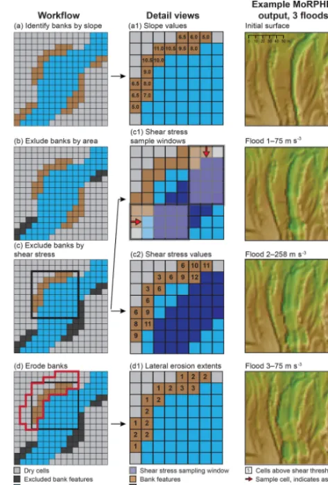
To begin, the model calculates the slope of all cells in the model domain; all simulations presented herein used a cell resolution of 2 m (Rees River; Sect. 3.1) or 1 m (River Feshie; Sect. 3.2). The relatively coarser cell resolution on the Rees was chosen for computational efficiency, particularly with re-gard to the hydraulic modelling component of MoRPHED, as the Rees site encompassed a considerably larger spatial do-main than that of the Feshie. Cells that exceed a user-defined slope criterion, which was set to 7 % by examining the aver-age slope of cells that underwent bank retreat in field surveys for all simulations presented herein (Fig. 2a), are then identi-fied as candidate cells for undergoing bank erosion. Whether
Figure 2.Lateral migration algorithm schematic.
For each cell within these groups, the bed shear stress in the surrounding cells was sampled using a 3×5 neighbour-hood window oriented in the cardinal direction of the candi-date cell’s aspect. The bed shear stress values in these cells were then averaged, producing a single shear stress value for the delineated group of cells. Those cell groups with aver-age shear stress below a user-defined criterion, here set to 50 N m−2, were excluded. The use of near-bank shear stress as a predictor variable for estimating lateral bank retreat has been applied by numerous researchers, including Ikeda et al. (1981), Howard (1992, 1996), Sun et al. (1996).
The cells that remained were those exceeding both the slope and near-bank shear stress thresholds; and for each of these cells, the model then removed material from a num-ber of adjacent cells specified by Eq. (11) and shown in Fig. 2d1, which computes the lateral extent of bank erosion (n), rounded to the nearest whole cell, shown in Fig. 2d, as a function of slope (S) and near-bank shear stress (τ; Fig. 2d):
n=round
τ
3+1
∗S 15
. (11)
The location of thesencells was determined by moving away from the initial candidate cell at 1-cell increments in a di-rection opposite to the initial candidate cell’s cardinal aspect direction (i.e. simulating lateral bank retreat moving away from the channel). The number of cells adjacent to the ini-tial candidate cell is shown in Fig. 2d. All delineated cells were then surrounded by a 3×3 neighbourhood window, and the full group of candidate cells at the conclusion of this de-lineation routine is shown by the red polygon in Fig. 2d1. Within each of these 3×3 neighbourhoods, all cells were re-duced in elevation to a level equal to that of the lowest cell in the neighbourhood (sensu Nicholas, 2013b), and eroded sediment was immediately transported downstream and de-posited in a manner identical to that described below for bed transport and deposition.
Bank erosion and bank material transport and deposition are computed prior to bed morphodynamics (Fig. 1); and to conserve computational overhead, hydraulics are not recom-puted between these steps; as a result, bed scour is not altered in areas proximal to eroding banks. Further, because candi-date cells for bank erosion are identified simply on the basis of slope and shear stress, it is possible that cells away from the wet/dry boundary (i.e. the channel bed) can undergo ero-sion in this manner as well. We believe this approach is ap-propriate here as hydraulics and morphodynamics are com-puted only once per flood (at peak discharge); and as such, steeply sloping cells susceptible to erosion may be inundated within the channel at the event peak, but may still undergo subaerial failure on the rising or falling limb of the hydro-graph. We note that Eq. (11) was used for simulations on both river systems studied here, which varied considerably in their constituent volumes of fine/cohesive sediment and vegetation extent (see Sect. 3). Thus, these values are likely applicable for a variety of rivers, but we caution that for
sys-tems with exceptional bank cohesion, whether via vegetation or fine sediment, adjustment of these parameters may be nec-essary. Finally, as opposed to a physically based relationship between shear stress, bank slope, and the extent of lateral erosion, Eq. (11) was derived through qualitative calibration; that is, rather than presenting a deterministic methodology for quantifying bank retreat, this approach is simply reflec-tive of the best qualitareflec-tive correspondence between mod-elling results and field observations of areas undergoing bank erosion.
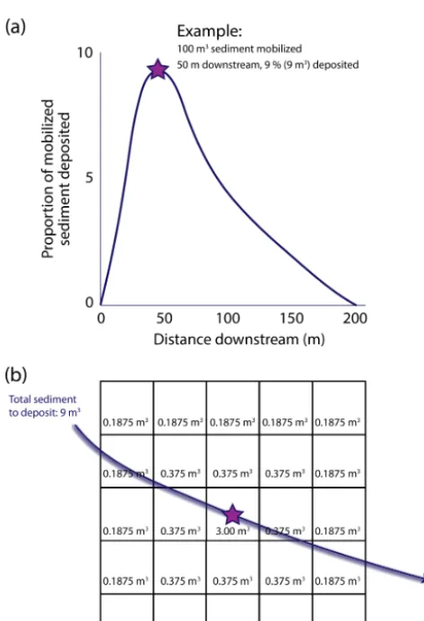
2.4 Bed or bank sediment transport and deposition Once entrained, bed or bank sediment is mobilized down-stream along flow lines which are delineated using velocity vectors from Delft3D. Although MoRPHED is inherently a cell-based (i.e. raster) model, Delft3D-derived velocity vec-tors did not necessarily pass through the centre of any given cell within the MoRPHED model grid. To account for this, the nearest grid cell was computed along the Delft3D ve-locity vectors at downstream intervals equal to the compu-tational domain cell size (i.e. 1 m on the Feshie, 2 m on the Rees; see Sect. 3). In the field, deposition of sediment consis-tently occurs in diffuse patterns, such as “tear-drop” forms of lobate bars, prograding bedload sheets, and thinly mantled overbank deposits (Ashmore, 1982; Ferguson and Werritty, 1983; Wheaton et al., 2013). To mirror this diffuse deposi-tion, the model distributes sediment within a 5×5 window of cells surrounding the candidate deposition cell, with the can-didate cell receiving 1/3 of the deposited sediment, the adja-cent 8 cells receiving 1/3 of the deposited sediment between them, and the outer ring of 16 cells receiving the final 1/3 of deposited sediment. In the case of dry cells that occur in the 5×5 neighbourhood, the dry cell(s’) sediment is divided among the population of wetted cells in the neighbourhood. The total volume of deposited sediment within this 5×5 win-dow is equal to the fraction of all entrained sediment from upstream given by a user-defined path-length distribution at the centre cell’s distance downstream from the entrainment location (Fig. 3).
text file. Because sediment deposition is simply computed via a provided path-length distribution (and particles are not dynamically tracked on their journey downstream), sediment transport effectively occurs instantaneously in the model. As such, a key assumption within MoRPHED is that modelled events are of sufficient duration to allow particles to transit the full length of the specified path-length distribution. Lab-oratory results of braided gravel-bed rivers have, however, indicated that particle transport and deposition, and develop-ment of a path-length distribution, occur quite rapidly after the onset of competent flow (see Kasprak et al., 2015). At any given cell within the model domain, elevation change is computed as the difference between erosion and deposition at that location. It is possible for any particular cell, over the course of a model run, to experience erosion exclusively, de-position exclusively, both erosion and dede-position, or a total lack of sediment scour and deposition.
2.5 Sediment import and export
For each simulated event, the model tracks the volume of sed-iment passing the downstream or lateral reach boundaries. In effect, export of sediment occurs when the length of the user-specified path-length distribution exceeds the downstream or lateral boundaries of the model domain. When this occurs, the remaining volume of sediment (the amount of eroded sediment not yet deposited along the flow line) is recorded as having been exported from the reach. Sediment import is user-specified and can be (a) set equal to the volume of sed-iment export during the preceding event (e.g. sedsed-iment equi-librium; Grams and Schmidt, 2005), (b) specified as a percent of sediment export during the preceding event, or (c) speci-fied via a text file detailing absolute volumetric sediment im-port during each event (e.g. sedigraph time series). Algorith-mically, the model computes flowpaths from each wetted cell at the upstream reach boundary and distributes the total vol-ume of imported sediment to each cell of each flowpath as specified in the user-input path-length distribution. Sediment is introduced to the reach at the end of each event (Fig. 1; i.e. following hydraulic and bed or bank morphodynamic modelling) and prior to initiation of the subsequent event, as this allows for the import of sediment once exported sedi-ment volumes are known. Sedisedi-ment leaving the lateral reach boundaries was included in the total export volume, along with sediment leaving via the downstream reach boundary.
2.6 Model verification
To compare the outputs of the model with field-based surveys of channel evolution, we derived several morphometric pa-rameters along with comparing DEMs of difference (DoDs) and contributions of individual braiding mechanisms to total geomorphic change. Each of these three verification compo-nents are discussed below.
2.6.1 Morphometric indices
We manually quantified the braiding index (IB) for the initial
and final field surveys and model runs of each simulation de-scribed here. Braiding index was computed by averaging the number of channels across five evenly spaced transects along the length of the model domain (Howard et al., 1970; Egozi and Ashmore, 2009). Channels were defined by wetted areas as modelled using Delft3D at estimated baseflow for each modelling site. In addition, we measured the total sinuosity (ST) of the modelled reach for the first and last model runs
in each system. Total sinuosity (Richards, 1982) was defined by the ratio of the length of all anabranches (LA) compared
to the down-valley length of the model domain (LD):
ST= LA LD
. (12)
Finally, we computed the number of confluences, diffluences, and channel heads for initial and final field and model DEMs. The procedure for delineating confluences, diffluences, and channel heads is detailed by Wheaton et al. (2013). In brief, it requires manual location of areas where one anabranch splits into two anabranches (a diffluence), areas where two anabranches join to form one anabranch (a confluence), and locations where small side channels or chutes begin (a chan-nel head). In theory, the number of confluences should be roughly equal to the number of diffluences plus the number of channel heads for a braided river. Instances where dif-fluences and channel heads outnumber condif-fluences are in-dicative of distributary systems (e.g. deltas; Jerolmack and Mohrig, 2007), while sites dominated by confluences are indicative of dendritic networks that collect low-order flow paths into a few main channels.
2.6.2 DEMs of difference (DoDs)
Figure 3.Particle transport and deposition routine. Panel(a)shows computation of the proportion of sediment to deposit as a function of eroded sediment via a particle path-length distribution,(b)shows the neighbourhood window approach for averaging deposited sediment over adjacent cells.
Figure 4.Path-length distributions used in MoRPHED modelling on(a)the River Feshie and(b)the Rees River. Peak of the distri-butions corresponds to average along-flow spacing between conflu-ence and diffluconflu-ence pairs.
threshold of±0.2 m to better visualize and delineate braid-ing mechanisms and to account for the larger magnitude ele-vation changes that occurred over wide swaths of the
braid-plain over this extended timescale. While this simple thresh-old value method is not necessarily the most robust method available for modelling error in field-surveyed DEMs, those DEMs output from the model do not contain survey error as would be expected from field-based DEMs. As such, a simple minLoD of 0.10 m allowed us to use identical error modelling methods to directly compare areas of change in field and modelled DoDs while simultaneously removing a great deal of the survey noise and uncertainty present in field DEMs, along with removing extremely low-magnitude ele-vation changes in modelled DEMs.
From DoDs, we extracted elevation-change distributions (ECDs, a histogram of all volumetric changes), along with deriving the net sediment imbalance during each survey and model period (the percent departure of the sediment budget from equilibrium conditions).
2.6.3 Braiding mechanisms
sites (Wheaton et al., 2013; Kasprak et al., 2015; Sankey et al., 2018a, b), and efforts aimed at the automated mechanistic segregation of geomorphic change have also been presented in the literature (Kasprak et al., 2017). This classification al-lowed us to compute and compare the volumetric contribu-tion of each braiding mechanism to total geomorphic change in both field and model-derived DoDs.
3 Study sites
3.1 Rees River, South Island, New Zealand – event and annual scales
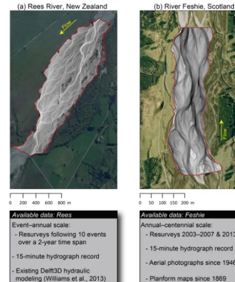
The braided gravel-bedded Rees (Fig. 5) drains a 402 km2 catchment of the uplifting metasedimentary Southern Alps and flows into Lake Wakatipu. The 2.5 km study reach is an actively braided channel which flows through a deglaciated valley, and the river is braiding in response to sediment de-livery from the tectonically active landscape (Williams et al., 2013). The hydrology of the system is dominated by a re-sponse to both seasonal snowmelt and rainfall, and under-goes floods in the spring, summer, and autumn that may completely alter the morphology of the braidplain over the course of a single flood. A temporary gauging station at In-vincible (6 km upstream of the study reach) operated from 2009 to 2011 and is used to drive hydraulic components of the model. Mean discharge during the 2010 and 2011 hy-drological years was 20 m3s−1, with a maximum flow of 475 m3s−1(Williams et al., 2015). The survey data on the Rees include 0.5 m resolution DEMs constructed via a fu-sion of terrestrial laser scanning (TLS) and optical-empirical bathymetric mapping surveys (Williams et al., 2014), which were downsampled to 2 m resolution for modelling. In total, 10 floods ranging from 51 to 403 m3s−1 were captured as part of the ReesScan project (Brasington et al., 2012) from 2009 to 2011, with post-flood DEMs surveyed in the period between each high flow. These pre- and post-flood DEMs, along with a continuous hydrologic record and a high degree of dynamism across the braidplain at the event scale make the Rees an ideal candidate to examine the performance of the model at the event and annual scales.
3.2 River Feshie, Scotland – annual and decadal scales The weakly braided gravel-bedded Feshie (Fig. 5) is a trib-utary of the Spey River and drains 231 km2of mountainous, postglacial terrain. Underlain by metamorphic and igneous rocks, the basin ranges from 230 to 1260 m in elevation. The mean flow near the river’s outlet was reported by Ferguson and Werritty (1983) as 8 m3s−1withQ5=80 m3s−1.
Topo-graphic data for the 1 km study reach of the Feshie consist of 9 years of resurveys (2000, 2002–2008, 2013) comprising more than a decade of channel change using RTK-GPS (real-time kinematic GPS, 2000–2006) along with TLS and RTK-GPS fusion scans performed for three surveys (2007–2008,
Figure 5.Morphodynamic modelling sites. Overview maps of Rees River(a)and River Feshie(b). Hill-shaded DEMs (2 m resolution for Rees and 1 m resolution for Feshie) are shown atop aerial pho-tograph base layers. Information on data availability for both sites are shown in lower panels.
4 Results
4.1 Hydraulic model calibration 4.1.1 Rees River
Because we modelled the same reach of the Rees previously analysed by Williams et al. (2013), we simply used the values ofks(0.10) andυ(0.10) obtained in that study (Table 1). We
found that these values resulted in good agreement between field-measured and modelled water depth, velocity, and inun-dation extents. The reader is referred to Williams et al. (2013) for more detailed analysis of the validity of Delft3D on the Rees (and in braided gravel-bed rivers in general).
4.1.2 River Feshie
In contrast to the Rees, no comprehensive validation and ver-ification of Delft3D exists on the Feshie; as such, we lever-aged existing surveys of wetted areas from 2003 to 2007 in concert with surveyed water depth in those years to ex-amine the performance of Delft3D. Because field surveys were conducted at low flows to facilitate rapid measurement of braidplain topography, here we are only able to verify the results of Delft3D at these low flows. However, Delft3D has been employed and verified on braided gravel-bed rivers at the flood stage (Javernick, 2013), demonstrating that the model can accurately reproduce flood-stage hydraulic fea-tures and can be used to drive morphodynamic evolution at the event-scale. For modelling on the Feshie, we esti-mated discharge by downscaling the average observed flow for the relevant survey period at the nearest gauging station (Scottish Environment Protection Agency no. 8013, Feshie at Feshiebridge) located approximately 11 km downstream using an empirically derived discharge-area coefficient of 0.71 (Wheaton et al., 2013). The value of discharge taken at Feshiebridge was the average flow during each year’s sur-vey period (average of 2 weeks). We estimated the down-stream water elevation using surveyed inundation extent in combination with the DEM for each year modelled. Down-stream water surface elevation estimated from the spatial data were cross-checked using a reach-scale conveyance calcula-tion (Williams et al., 2013).
Results of our validation of Delft3D on the Feshie at low flow are shown in Fig. 6. Here we report (a) the mean of depth differences between modelled and observed values (Ddiff), along with (b) the congruence of the modelled and
measured inundation extents (Fc; Bates and De Roo, 2000)
as described by the ratio of intersection and union areal ex-tents. These two metrics are described by Eqs. (16)–(17).
Figure 6.River Feshie hydraulic modelling. Surveyed water sur-face extent in each of the five years (2003–2007) was compared to modelled inundation extent in the same years using discharge lev-els approximated using data from the gauge at Feshiebridge. Areas observed (but not predicted) to be inundated shown in blue, areas predicted (but not observed) to be inundated shown in green. Areas which were correctly predicted as being inundated shown in red. Base layer is a hill-shaded 1 m DEM.
Ddiff= n
P
i=1
xmod−xobs
n (13)
FC=
IAobs∩IAmod
IAobs∪IAmod
·100 (14)
The metrics indicate that at low flow, Delft3D accurately predicted both depth and inundation extent across the Fes-hie study reach. BothDdiff andFc are consistent with
val-ues obtained by Williams et al. (2013) on the Rees (mean Ddiff=0.04, meanFc=81.2 on the Feshie) and are
indica-tive of a good agreement between hydraulic predictions and field-observed flow characteristics, despite the empirically scaled discharge.
Table 1.Delft3D hydraulic modelling parameters.
Sim. Time Cell D84 Colebrook–White Eddy viscosity
Site time (h) step (s) size (m) Nodes (m) roughness (ks) (υ, m2s−1)
Rees 1 0.025 2 352 231 0.035 0.10 0.1
Feshie 1 0.025 1 201 116 0.1 0.29 0.1
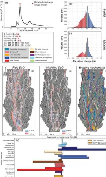
heavy rainfall in the upstream watershed (Fig. 7). Peak flows reached a maximum instantaneous discharge of 259 m3s−1 at the upstream Invincible gauging station during the after-noon of 9 December. Two smaller peaks in the hydrograph of 75 m3s−1(afternoon of 8 December and morning of 12 De-cember) also occurred during this event. Our modelling em-ployed a single representative grain size (D50) of 20 mm. We
used an equilibrium sediment budget condition for this sim-ulation (Sect. 2.5). Geomorphic change captured by pre- and post-flood TLS revealed that the most volumetrically sig-nificant mechanisms of change were transverse bar conver-sion (22 %), bank eroconver-sion (21 %), and lobe dissection (19 %). Qualitatively, event-scale dynamics across the study reach are marked by widespread geomorphic change, particularly in the centre of the braidplain where development of a single main channel occurred via channel incision, bank erosion, and avulsions of smaller anabranches leading to deposition and subsequent dissection of mid-channel bars. Geomorphic change on the edges of the braidplain was somewhat muted, consisting largely of infilling of anabranches and accretion of central bars. Field-surveyed elevation changes ranged from −1.70 to +1.32 m (Fig. 7d). The braiding index (IB)
de-creased from 3.6 to 2.0 following the flood, and total sinu-osity (ST) decreased from 4.5 to 2.9.
Results of morphodynamic modelling on the Rees for this event are shown in Fig. 7. This event-scale model was run using a steady-state discharge of 259 m3s−1as seen in the December 2009 flood peak. Total model runtime for the single event was approximately 90 min. Modelled elevation changes in the study reach ranged from−1.76 to+0.89 m (Fig. 7e); these and subsequent modelling results incorpo-rate a 0.1 m minLoD (i.e. threshold) as discussed in Sect. 2.6. Overall, geomorphic change was concentrated near the cen-tre of the braidplain, similar to geomorphic change measured from field data. Large swaths of bank erosion along a cen-tral anabranch developed, although not to the extent seen in field data. In general, geomorphic change in the modelled DoD appears muted in comparison to the field-based DoD. This is reflected in the ECD shown for field and model data on the Rees (Fig. 7c), particularly with regard to the erosional component of volumetric change (47 598 m3in the field com-pared to 20 663 m3in the model; Table 2). Similarly, depo-sitional volumes were greater in the field (35 551 m3) com-pared to those in the model (16 188 m3; Table 2). On av-erage, erosion depth across the study reach was 0.13 m as observed through field measurement and 0.07 m when
mod-elled. Deposition averaged 0.10 m in the field and 0.06 m in the model (Table 2). The most volumetrically significant braiding mechanisms in this run were central bar develop-ment (25 % of total volumetric change), bar edge trimming (16 %), and bank erosion (15 %).
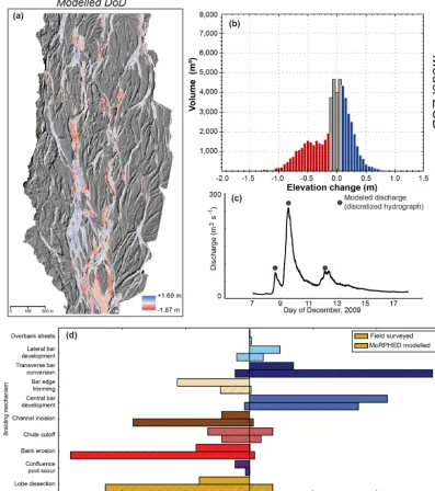
Case study: hydrograph discretization
The choice of model time step is one of the more impor-tant considerations in morphodynamic modelling, whereby the user must strike the optimal balance between a model time step fine enough to preserve computational stability and which is coarse enough to allow computation over meaning-ful timescales (Brasington et al., 2007). To investigate these questions using MoRPHED, we discretized the hydrograph used in event-scale modelling on the Rees so as to model three discrete points over the course of the modelled flood (Fig. 8). These discharges were 75, 259, and 75 m3s−1 or
the three points. Note that in this case study we did not al-ter the time step of the model itself, which remained at the event scale, but rather computed morphodynamic change at three instances over the course of a multi-day flood with three sub-peaks using an equilibrium sediment budget. Plan-form DoD, ECD, and volumetric contribution of individual braiding mechanisms from this discretized model run are shown in Fig. 8. In general, morphologic changes were more widespread across the braidplain in the case of the discretized hydrograph modelling run than the single peak discharge hy-drograph (Fig. 8), with overall area of change increasing, yet still smaller than field-observed change volumes (157 504 m2 in the model compared to 287 184 m2in field data; Table 2). The ECD from this model run more closely approximated the field-derived ECD, with low-magnitude elevation changes (e.g.<1 m) dominating the change distribution (Fig. 8).
4.3 Annual-scale morphodynamic modelling: River Feshie
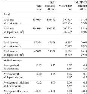
Table 2.Rees River event modelling: geomorphic change detection results; results of discretized modelling shown initalics.
Field MoRPHED
Field threshold MoRPHED threshold raw (0.1 m) raw (0.1 m)
Areal
Total area 435 604 146 472 390 555 57 387
of erosion (m2) 418 856 63 496
Total area 461 084 140 712 500 233 85 160
of deposition (m2) 389 072 94 008
Volumetric
Total volume 57 324 47 598 28 297 20 663
of erosion (m3) 28 679 20 291
Total volume 47 022 35 551 28 102 16 188
of deposition (m3) 28 130 19 480
Vertical averages
Average depth 0.13 0.32 0.07 0.36
of erosion (m) 0.07 0.32
Average depth 0.10 0.25 0.06 0.19
of deposition (m) 0.07 0.21
Average total thickness 0.12 0.09 0.06 0.04
of difference (m) 0.07 0.05
Average net thickness −0.01 −0.01 0.00 −0.01
of difference (m) 0.00 0.00
documented that flows of 20 m3s−1were indeed competent for bed material in the study reach, albeit without full mo-bility of all bed particle sizes. Our modelling on the Feshie employed a single representative grain size (D50) of 50 mm.
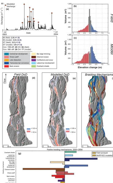
Wheaton et al. (2013) noted that the most volumetrically significant braiding mechanisms during the 2003–2004 pe-riod were chute cutoff (29 %), bank erosion (16 %), and chan-nel incision (15 %). Overall, geomorphic change was primar-ily confined to a main channel bisecting the braidplain lon-gitudinally, with one anabranch on the left side of the braid-plain undergoing bank erosion and central bar development. Braiding index (IB) during the 2003–2004 epoch increased
from 1.8 to 2.8, and total sinuosity (ST) also increased from
2.5 to 3.5. Results of morphodynamic modelling are shown in Fig. 9e. Total model runtime for the series of 12 events modelled during the 2003–2004 period was approximately 6 h. The results of DEM differencing are shown in Table 3. Elevation changes in the modelled reach ranged from−1.25 to+1.49 m. Overall, geomorphic change was marked by the accumulation of transverse bars and the development of cen-tral bars throughout the model reach, along with incision of a central anabranch. Sculpting or trimming of central bars (Fig. 9f; e.g. Wheaton et al., 2013) was also prevalent. The most volumetrically significant braiding mechanisms
dur-ing this model run were channel incision (26 %), transverse bar conversion (20 %), and central bar development (14 %). Overall, geomorphic change predicted via modelling was greater than that observed from field data (Table 3). However, both field and model ECDs (Fig. 9b, c) depict change distri-butions wherein the greatest volume of geomorphic change is the result of low-magnitude elevation changes. The average depth of elevation changes were generally well predicted by the model, although average erosion and deposition depths were over-estimated by 0.02 and 0.03 m, respectively (Ta-ble 3).
Case study: contrasting path-length distributions
an-Figure 8.Rees River discretized hydrograph case study. DoD from MoRPHED modelling shown in(a), with ECD in(b), event hydrograph with model points shown in(c), and volumetric contribution of braiding mechanisms in field and model shown in(d). Refer to field-based results shown in ECD(b)and DoD(d)in Fig. 7 for comparison.
nual hydrograph on the River Feshie in a manner identical to Sect. 4.3, except we varied the characteristics of the speci-fied path-length distribution (Fig. 10). We employed a com-pressed Gaussian distribution (Fig. 10a), a flattened Gaussian distribution (Fig. 10b), and an exponential-decay-type distri-bution (Fig. 10c; Pyrce and Ashmore, 2003b); each of these distributions had a total length identical to our original distri-bution on the Feshie (Fig. 10a). We also modelled two short-ened distributions (length=50 m): a shortened Gaussian dis-tribution (Fig. 10d) and a shortened exponential disdis-tribution (Fig. 10e). As previously stated, we assume that event
du-ration is sufficient for particles to transit the full length of the specified path-length distribution, and in all simulations we employed an equilibrium sediment budget (Sect. 2.5) where the amount of imported sediment was set equal to that amount crossing the downstream and lateral model bound-aries.
Table 3.River Feshie annual modelling, geomorphic change detection results.
Field MoRPHED
Field threshold MoRPHED threshold raw (0.1 m) raw (0.1 m)
Areal
Total area of erosion (m2) 66 074 9970 50 021 17 444
Total area of deposition (m2) 49 998 7236 58 366 20 263
Volumetric
Total volume of erosion (m3) 4433 2806 6149 5239
Total volume of deposition (m3) 2704 1543 5986 4910
Vertical averages
Average depth of erosion (m) 0.07 0.28 0.12 0.30
Average depth of deposition (m) 0.05 0.21 0.10 0.24
Average total thickness of 0.06 0.04 0.11 0.09 difference (m)
Average net thickness of −0.01 −0.01 0.00 0.00 difference (m)
vealed that while the compressed and stretched Gaussian dis-tributions were marked by more laterally extensive deposi-tion at higher magnitudes (e.g. ∼1 m), the exponential and two shortened distributions (Fig. 10c–e) generally contained depositional signatures marked by numerous low-magnitude (e.g. 1z <0.5 m) changes. The same is true for the ero-sional component of elevation change, with compressed and stretched Gaussian distributions marked by a wide range of erosional elevation changes up to and exceeding 1 m, whereas the exponential and shortened distributions gener-ally displayed erosional changes less than−1 m in depth.
4.4 Decadal-scale morphodynamic modelling: River Feshie
We modelled morphodynamics during the 10-year period be-tween July 2003 and June 2013 along the River Feshie. The estimated hydrograph at Glen Feshie during this period is shown in Fig. 11a; and using an equilibrium sediment bud-get, we modelled all peaks above 20 m3s−1as described in Sect. 3.2 and in Wheaton et al. (2013) for a total of 185 flood events ranging from 20 to 95 m3s−1.
Differencing DEMs from survey data at the beginning and end of the analysis period reveals elevation changes rang-ing from−2.4 to+2.1 m (Fig. 11d). DEM differencing in-dicates that the study reach underwent slight net aggrada-tion (+3.6 % imbalance). The most volumetrically signifi-cant braiding mechanisms during this time period were the development of central bars (25 % of volumetric changes), transverse bar conversion (17 %), and bank erosion (16 %). As the relative contribution of individual braiding mecha-nisms may be misleading at decadal scales due to signature overprinting and hence difficulty in interpretation of braiding mechanism, we note that over a 5-year period (2003–2007; Wheaton et al., 2013) on the Feshie the most volumetrically significant braiding mechanisms were chute cutoff (24 %), bank erosion (20 %), and transverse bar conversion (19 %). Braiding index (IB) during the 2003–2013 epoch increased
from 1.8 to 2.4, and total sinuosity (ST) also increased from
2.5 to 2.9 (Fig. 11).
Results of morphodynamic modelling from 2003 to 2014 are shown in Fig. 11e. Total model runtime for the 185-flood series was approximately 72 h. Geomorphic change ranged from+2.1 to−8.07 m (Fig. 11e). A mask was employed to exclude areas of the reach<25 m from the upstream bound-ary, as boundary artefacts resulting from the use of point dis-charges in the Delft3D model produced high magnitudes of geomorphic change (e.g. >5 m) in these areas. While geo-morphic change in the field was marked by generally thin-mantled erosion and deposition across the braidplain, the model produced more widespread, high-magnitude erosional change (Table 4). While the depositional component of the ECD produced by the model generally characterized that of the field-derived ECD (Fig. 11b, c), the model predicted a smaller area, but greater volume, of scour (Table 4). The
model generally reproduced the form and magnitudes of de-position seen in the field, but the lowest-magnitude deposi-tion (e.g.<0.5 m) was more volumetrically significant in the field than in the model. While the model did produce avul-sion (i.e. the development and inciavul-sion of a new channel on the left-hand side of the upstream end of the braidplain in Fig. 11), it did not produce avulsion in the same locations seen in the field, nor with the same frequency, as evidenced by the model predicting an incised, simplified channel net-work in 2013; this downcutting behaviour was also seen by Singh et al. (2017) in decadal-scale morphodynamic mod-elling using Delft3D. This central anabranch incision was accompanied by a reduction in channel nodes (confluences, diffluences, and channel heads), and thus a simplified chan-nel planform in the model as compared to the field dataset (Fig. 11). The most volumetrically significant braiding mech-anisms during the 2003–2013 model run were central bar de-velopment (27 %), transverse bar conversion (22 %), and lobe dissection (1 %). In addition, the role of bar edge trimming (8 %), a process treated identically to bank erosion in MoR-PHED, was magnified compared to field-derived mechanistic segregation (2 %), as was the role of channel incision (11 % in the model as compared to 7 % in the field).
5 Discussion
We developed a morphodynamic model that computes sed-iment transport according to user-specified path-length dis-tributions, and subsequently employed this model to pre-dict channel evolution at two braided river reaches across timescales ranging from a single event to a decade. We ob-served that the model reproduced many of the geomorphic changes observed in the field, although the magnitude and mechanisms of those changes often diverged from observa-tions using field data. At the same time, the modular design of the modelling framework may hold promise for explo-ration of braided channel evolution, and also raises questions regarding the way processes are algorithmically represented and the model’s sensitivity to those process representations.
5.1 Emergent versus parameterized processes
Table 4.River Feshie decadal modelling, geomorphic change detection results.
Field MoRPHED
Field threshold MoRPHED threshold raw (0.2 m) raw (0.2 m)
Areal
Total area of erosion (m2) 38 332 23 836 48 092 23 542
Total area of deposition (m2) 70 329 36 045 57 087 26 861
Volumetric
Total volume of erosion (m3) 13 944 12 680 25 134 23 744
Total volume of deposition (m3) 18 264 14 677 15 712 13 748
Vertical averages
Average depth of erosion (m) 0.36 0.53 0.52 1.01
Average depth of deposition (m) 0.26 0.41 0.28 0.51
Average total thickness 0.30 0.25 0.39 0.36 of difference (m)
Average net thickness 0.04 0.02 −0.09 −0.10 of difference (m)
be simply captured by an excess shear stress scour approach (Eq. 7; Sect. 2.2).
The geomorphic changes that the model most commonly produce are those that result from focused scour and lon-gitudinally continuous deposition, given the nature of the scour and deposition functions used in the model. In par-ticular, channel incision, bar edge trimming, bank erosion, and lateral or central bar development are common processes produced by the model (Figs. 7, 9, 11). Additionally, given the single-peaked Gaussian distributions used herein, those braiding mechanisms which involve deposition immediately downstream of an erosional source are difficult to reproduce. For example, Wheaton et al. (2013) demonstrated the impor-tance of chute cutoff as a braiding mechanism on the Fes-hie, noting that chute development across point bars not only manifested as erosion, but that the scoured material was often deposited immediately downstream of the chute. Similarly, scoured bank material (e.g. mass failures) may often be de-posited at the bank toe rather than transported downstream. In both cases, the model makes no differentiation in trans-porting the eroded sediment, mobilizing the material accord-ing to the user-specified path-length distribution; as such, proximal couplets of erosion and deposition are difficult to reproduce in the model. Finally, we note that chute cutoff in the model always occurred in locations of pre-existing chutes across point bars. Because chute cutoff often occurs at the falling stage of floods, when braidplain-inundating flows are first being confined into anabranches, our model may not properly reproduce chute cutoff as a result of only comput-ing peak flood hydraulics, and averagcomput-ing shear stress across
a range of model cells. Although headward erosion of these pre-existing chutes typically occurred in the model, thus in-creasing their extent, we did not observe any instances where chute cutoff was initiated in the model without an existing chute or channel head being present on a bar surface. As such, chute cutoff may represent a braiding mechanism that must be explicitly included in the model’s code in order to be properly represented in the future.
over-scouring of the bed, and provide greater fidelity to field observations of channel morphodynamics when modelling at decadal and longer timescales.
5.2 Sensitivity to process representation 5.2.1 Hydrograph discretization
In Sect. 4.2.1, we modelled a single event on the Rees as three discrete discharges on the hydrograph (Fig. 8). Because MoRPHED under-predicted the volume of change, partic-ularly due to the absence of low-magnitude scour, during the single-event simulation (Fig. 7), we sought to under-stand whether discretizing the hydrograph would allow for an improved prediction of overall volumetric change, and low-magnitude erosional change in particular. Overall, dis-cretizing the hydrograph into three modelling time steps only marginally increased predictions of volumetric change across the study reach: total volumetric change in the discretized run (Fig. 8) was 39 771 m3 compared to 36 851 m3 in the single-event model run (Fig. 7). Both modelling approaches underestimated the amount of volumetric change in the field (83 149 m3).
Discretizing the hydrograph also increased the amount of low-magnitude scour predicted by the model (Fig. 8b), more accurately reflecting the field-derived ECD (Fig. 7b). It is likely that this is the result of the 0.1 m elevation threshold used in our change detection (Sect. 2.7.2), whereby additive changes due to erosion largely did not exceed 0.1 m depth after a single flood event, but did exceed this threshold when three discrete hydrograph points were measured. Whereas erosional processes that lead to high-magnitude scour, such as bank erosion, dominated the ECD in the single-event model run, processes such as channel incision and lobe dis-section were more prevalent in the discretized hydrograph model run. Additionally, several areas of high-magnitude bank and bar trimming were largely offset by deposition of imported or scoured material during the discretized hydro-graph run, thereby decreasing the overall magnitude of scour in those areas (Fig. 8b).
5.2.2 Path-length distribution
We modelled annual-scale morphodynamics on the Feshie using five different path-length distributions (Sect. 4.3.1). There is overall similarity between the DEMs produced by the model (and hence the DoDs shown in Fig. 10) using these distributions, yet subtle differences may reflect the dis-tinct nature of the spatial arrangement of erosion and depo-sition. Overall, the similarity between the modelled distri-butions may also be the result of the smoothing algorithms used in the model to ensure computationally stable output surfaces, such as the along-flow averaging of shear stress and neighbourhood windows used for deposition (Sect. 2.4), both of which may act to reduce the variability introduced by the choice of a particular path-length distribution.
In fluvial settings, erosional processes typically operate over small spatial scales (e.g. bank erosion, bar trimming, pool scour), and the magnitude of scour in these focused areas is typically higher than diffuse, broad-scale deposi-tional processes such as overbank sheets or accretion of mid-channel or lateral bar material (Wheaton et al., 2013). As such, we suggest that the overall similarities, as well as the differences, between our model’s outputs using these con-trasting path-length distributions reflects the ability of de-position to counterbalance elevation changes due to scour of material, and the fact that the diffuse nature of the path-length distributions used here make this counterbalancing difficult. For example, the compressed and stretched Gaus-sian distributions (Fig. 10a, b) are both marked by broad ar-eas of erosion and deposition typically falling between±1 m in elevation change. However, high-magnitude areas of ero-sion are more rare, yet still present, in the stretched Gaus-sian distribution, which may be due to the more longitudi-nally extensive deposition of scoured material partially off-setting elevation changes due to erosion. The compressed and stretched Gaussian distributions stand in contrast to the ex-ponential and shortened distributions (Fig. 10c–e), where el-evation changes are largely confined between±0.5 m, and overall are more fragmented across the model reach. This does not reflect a reduced magnitude of erosion as Eq. (7) was used in all cases to predict scour depth; rather, the frag-mented nature of elevation changes, along with the narrower range of those changes, is likely due to the propensity for de-position to offset erosional changes given the more focused nature of the path-length distributions in Fig. 10c–e. Never-theless, in all distributions used, the volume of material de-posited in a given cell following erosion upstream is always a fraction of that which was eroded. Using the distributions in Fig. 10 and the deposition smoothing window detailed in Sect. 2.4, the volume of deposited sediment falls between 0.4 % and 8 % of the volume which is eroded; and as such, erosion may outpace deposition in many cells.
5.2.3 Path-length modelling as compared to CA and CFD morphodynamics
ob-servations or CFD modelling, which were closely correspon-dent. The over-prediction by the CA model resulted from the sole reliance on bed gradient to route flow, as opposed to also incorporating the momentum components of the Navier– Stokes equations (Coulthard and Van de Wiel, 2012; Fon-stad, 2013). Given that MoRPHED employed CFD-driven hydraulics (Sect. 2.1), and given that the boundary condi-tions employed in that modelling were largely identical to those used by Williams et al. (2016b), we hypothesize that the hydraulic modelling component of our approach on the Rees was likely in agreement with previous CFD modelling efforts conducted there.
With regard to morphodynamics, we can compare the general results of Williams et al. (2016b), who simulated the event-scale evolution of the same Rees River study reach used here. During a flood with a peak discharge of 227 m3s−1that occurred over a 2-day period in April 2010
using Delft3D, Williams et al. (2016) computed 37 204 m3of scour, 27 692 m3of deposition, and a net sediment budget of −9331 m3, similarly restricting sediment calculations to ar-eas of elevation change greater than±0.1 m. Our own event-scale modelling of a 4-day flood with a maximum discharge of 259 m3s−1in December of 2009 produced an estimated 28 297 m3of erosion, 28 102 m3of deposition, and a net sed-iment budget of −195 m3. While these results are not di-rectly comparable, given that they were generated from mod-els of two separate floods with varying (although similar) peak magnitudes, durations, and antecedent channel form, the first-order agreement between the magnitudes of geo-morphic change for relatively similar event magnitudes vides evidence that our event-scale approach is able to pro-duce similar magnitudes of geomorphic change as seen in CFD modelling that utilizes an Exner-based approach (i.e. Eq. 6) for computing morphodynamic evolution. At the same time, divergence in the nature of geomorphic change between the two approaches is evident. While the majority of ele-vation changes computed by Williams et al. (2016b) were of low magnitude (e.g. ±0.1 m) with respect to both ero-sion and deposition, MoRPHED predicted that the majority of sediment scour was the result of focused high-magnitude erosion centred around −0.5 m (Fig. 7c). The depositional component of elevation change predicted by MoRPHED was marked by low-magnitude deposition comprising the major-ity of changes, in line with the results of CFD modelling from Williams et al. (2016a), thus suggesting that a path-length approach produces similar results with regard to deposition as compared to CFD morphodynamic modelling, whereas the computation of sediment scour on a once-per-event ba-sis likely requires refinement. Finally, the parameterization of bank erosion proved challenging in both MoRPHED and in the Delft3D simulations of Williams et al. (2016b) on the Rees, although for differing reasons. In the case of CFD mod-elling, disparities between field observation and model out-puts primarily arose due to differences in the positioning and migration direction of individual channels (see Williams et
al., 2016b, Fig. 7); whereas in MoRPHED, model outputs generally predicted channel deepening in lieu of migration (Fig. 7e). Within both CFD and event-scale modelling, these results emphasize the need for further investigation into the mechanics of intra-flood bank erosion and lateral migration of braided rivers as a function of both near-bank shear stress and slope of near-bank cells within the model domain. In par-ticular, Stecca et al. (2017) provide a framework for assess-ing the performance of non-cohesive bank erosion algorithms and apply this within a cross-sectional framework. The ap-plication of this framework to identify the most important behavioural algorithms for modelling bank erosion in two-dimensional simulations would be an appropriate next step to improve the model that is assessed here.
ap-proach, specifically the user-defined path-length distribution, is required at intra-flood timescales.
5.2.4 Imperfect models as exploratory tools
Models in the Earth sciences are necessarily imperfect (Oreskes et al., 1994), and the highly simplified nature of MoRPHED, combined with the highly dynamic and non-linear nature of braided river morphodynamics (Ashmore, 1991; Bristow and Best, 1993), implies that our model will necessarily fail to achieve perfect replication of field-observed geomorphic dynamics. However, even imperfect models can provide meaningful insight into the processes be-hind morphologic evolution of fluvial systems (Paola et al., 2009; Paola and Voller, 2005). MoRPHED is designed to fa-cilitate experimentation, particularly with regard to process inclusion or the particular aspects of process representation of bed and bank erosion, transport, deposition, and import dynamics (Fig. 1). For example, in Sect. 4.3.1, we explored the implications of altering the path-length distributions for bed and bank sediment transport or deposition, along with seeking to understand the advantages and drawbacks of dis-cretizing hydrographs during model runs. The notion of mor-phodynamic modelling that employs sediment transport rou-tines based on particle path-length distributions is in its in-fancy, and we have built the model as an exploratory tool that can be used to investigate the utility of this approach toward predictive modelling of braided river evolution. Several com-ponents of the model may be employed to investigate long-standing questions in our underlong-standing of braided river dy-namics, starting with the path-length approach itself. Recent field-based research on braided rivers has confirmed the cou-pled nature of sediment sources and sinks and the influence of sediment pathways on braiding maintenance (Williams et al., 2015). While it has long been hypothesized, and field and laboratory data have often confirmed, that mobilized parti-cles in braided rivers are preferentially deposited in associ-ation with regularly occurring channel bars (e.g. Pyrce and Ashmore, 2003a, b; Kasprak et al., 2015), the form of the path-length distribution, and its relationship to geomorphic unit spacing, is deserving of further study across braided sys-tems. As such, the choice of path-length distribution and sub-sequent comparison of model results with field observations may provide insight into the applicability of path-length dis-tributions on a system-by-system basis (Hassan et al., 2013). MoRPHED may also be used to investigate the utility of event-scale monitoring. Existing morphodynamic models typically employ a sediment continuity approach (e.g. Exner; Eq. 6), operating at very fine temporal scales, typically sec-onds to minutes. This approach produces results consistent with field observations (Bates et al., 2005), but comes at the expense of computational overhead, thereby restricting the timescales that can be modelled (Brasington et al., 2007). Because the time step of the model is, by default, a sin-gle event, computational resources are conserved, allowing
for extended simulations at annual and decadal timescales. However, it is unclear whether processes that occur over the course of a competent flow (e.g. avulsion, bank failures) can be adequately captured using an event-scale modelling ap-proach. In lieu of a continuity-based approach for comput-ing morphodynamic change, here we employed a simpli-fied event-scale estimation of bed scour depth as a function of flow hydraulics and bed sediment characteristics (Eq. 7, Sect. 2.2). At present, it is unclear whether this approach is valid across a wide range of river styles and/or indepen-dent of event duration; one potential way forward in model calibration may be to scale Eq. (7) such that field-observed changes, particularly those seen in ECDs at the event scale (Fig. 7), are matched as closely as possible, and then pro-ceeding with modelling over longer timescales. Such a model calibration approach was not attempted here, but may im-prove event-scale modelling fidelity in future work. Simi-larly, the degree to which a hydrograph may need to be dis-cretized and its constituent parts modelled (Sect. 4.2.1) to capture stage-dependent processes such as the development of chute cutoffs or bar edge trimming (Wheaton et al., 2013) is deserving of further investigation.
Finally, we note that the sequencing of individual floods may have implications for the geomorphic evolution of mod-elled reaches using this approach. For example, a large flood event may result in widespread scour of the reach and, un-der equilibrium sediment import parameters, may thus drive a large amount of bedload import and deposition at the up-stream end of the reach prior to the next event being mod-elled. The choice of path-length distribution used for im-ported sediment may further affect the degree to which large amounts of deposition could potentially occur at the up-stream model boundary, and the implications of these choices on model fidelity, although not explicitly evaluated here, deserve further study. Finally, although periodic sediment-supplying floods have been surmised to maintain the braided planform in lieu of continuous sediment supply, and thus may allow braided rivers to persist under conditions of sediment deficit at annual scales (Wheaton et al., 2015), the influence of flood sequencing on reach-scale morphodynamics has re-ceived relatively little attention in the literature and is de-serving of further work in the field as well as via numerical modelling.