Using Graph States for Quantum Computation and Communication

(1)

Communication

Thesis by

Kovid Goyal

In Partial Fulfillment of the Requirements for the Degree of

Doctor of Philosophy

California Institute of Technology Pasadena, California

2009

(2)

c

2009

(3)

(4)

Acknowledgements

I would like to start by acknowledging my thesis adviser, John Preskill, for giving me the freedom to pursue my interests and for setting a very high standard for me to aspire to. John has also provided the direction I needed at critical points in my career.

I would like to thank Robert Raussendorf for sharing a lot of his ideas with me and patiently explaining them when needed. Most of the great ideas in Chapter 2 were orig-inated by him. Robert has been a mentor and a guide.

I would like to thank Jim Harrington for introducing me to the numerical techniques needed for the analysis of the measurement based quantum computer and for writing relatively clear and easy to follow code.

I would like to thank Austin Fowler for asking me a lot of questions and thereby greatly improving the clarity and depth of my understanding. Austin also inspired me to make this work as clear and easy to follow as possible. The magic state distillation circuit diagrams and the CNOT gate construction in Chapter 2 are his.

I would like to thank Ben Toner, Panos Aliferis, Greg Ver Steeg and Prabha Mandayam Dodamanne for many stimulating discussions.

I would like to thank my parents, Ashima and Niraj, for supporting my desire to be-come a physicist and for providing me with a stimulating and enjoyable childhood.

I would like to thank my wife, Krittika, for being there and for sharing my love of physics.

(5)

Abstract

In this work, we describe a method to achieve fault tolerant measurement based quan-tum computation in two and three dimensions. The proposed scheme has an threshold of 7.8×10−3 _{and poly-logarithmic overhead scaling. The overhead scaling below the}

threshold is also studied. The scheme uses a combination of topological error correc-tion and magic state distillacorrec-tion to construct a universal quantum computer on a qubit lattice. The chapters on measurement based quantum computation are written in re-view form with extensive discussion and illustrative examples.

(6)

List of Figures

2.1 Birds eye view of computation . . . 9

2.2 The COPY operation . . . 9

2.3 The 2Dcluster state . . . 11

2.4 Schematic of a measurement based computer . . . 15

2.5 The cubic lattice for fault tolerant QC . . . 17

2.6 The schematicC3D . . . 20

2.7 2Dslice ofLp showing a logical qubit . . . 20

2.8 Mapping from slice to surface code . . . 21

2.9 Examples of correlation operators . . . 23

2.10 Error chains leave syndrome at their ends . . . 24

2.11 Initialization in theZ basis . . . 28

2.12 Initialization in theX basis . . . 29

2.13 Initialization of logical qubits in the|±θ〉state. . . 31

2.14 Pairing up the syndrome . . . 32

2.15 Correlation surfaces for the identity gate. . . 34

2.16 The correlation surfaces for theΛ(X)gate . . . 35

2.17 Circuits to perform non-Clifford gates . . . 36

2.18 Distillation circuits for|A〉and|Y〉 . . . 37

2.19 The logical cell . . . 38

2.20 Error chains as logical errors . . . 38

2.21 Example of a fault-tolerantΛ(X) . . . 40

2.22 Temporal order of operations in the bulk of the lattice . . . 41

3.1 Numerical simulation for the topological threshold . . . 46

3.2 Kappa dependence . . . 49

3.3 Operational overhead . . . 51

3.4 Operational overhead below threshold . . . 53

3.5 Qubit overhead . . . 54

3.6 Correlated errors inL . . . 55

3.7 Correlated primal and dual error chains . . . 57

4.1 Action of MCNOT . . . 60

4.2 Recurrence curves for the three-copy protocol . . . 63

4.3 The various purification protocols . . . 64

4.4 Trade-off curves for the different protocols . . . 70

(9)

List of Tables

1.1 Notation for common qubit operators . . . 7

2.1 Measuring a cluster qubit in the Pauli basis . . . 12

2.2 The duality transforms in two and three dimensions . . . 18

2.3 Notation for the components of the sub-latticesLp,Ld . . . 22

2.4 Relationships between correlations, syndrome, defects and errors . . . 27

2.5 Preparation and measurement ofX, Z . . . 30

3.1 Performance of magic state distillation . . . 50

(10)

List of Asides

2.1 The Stabilizer Formalism . . . 10

2.2 Graph States . . . 14

2.3 Fault tolerance . . . 17

2.4 Surface codes . . . 19

2.5 Homology onL . . . 25

(11)

Chapter 1 Introduction

As the components of computers have gotten smaller and smaller, quantum mechanical effects have begun to play an increasingly important role in the process. Traditionally, these quantum effects are classified as noise and efforts are made to minimize their ef-fects on the computation. However, in recent years it has been realized that exploiting these quantum effects can allow us to do a number of surprising and useful things, both in computation and communication.

1.1 Computation Powered By Quantum Mechanics

A classical computer (defined loosely as a computer that regards quantum effects as noise) represents data as bits, that is, as two level systems whose two levels are labeled by 0 and 1. Classical data consists ofbit strings, sequences of 0 and 1. The fundamental (and only) operation that a classical computer can perform on a single bit is to flip it. If there are two or more bits, the classical computer can in addition calculate their product or their sum. It is on this simple foundation that classical computation is built.

A quantum computer, on the other hand, represents data asqubits. A qubit is also a two level system, except that it is aquantumsystem. This means, in particular, that it can be in asuperpositionof 0 and 1. For a given set ofn bits, a classical computer can put them into only a single state out of the 2n _{possible states, whereas in a quantum}

computer they can be in a superposition of all 2n _{states at once. This is what gives}

quantum computers their power. Examples of qubits include: the spin of an electron, where the 0 and 1 states correspond to the up and down states of the electron spin along some predefined axis; photon polarization, where the 0 and 1 states correspond to left and right circularly polarized light; etc.

A qubit, which in general is in a superposition of 0 and 1 is represented by a state vec-tor: α|0〉+β|1〉; whereα, β are complex numbers satisfying the relation|α|2₊_|_β_|2₌_1.

(12)

entan-glement is difficult to achieve, roughly speaking, two quantum systems are said to be en-tangled when the state of the combined system cannot be described in terms of only the states of its two parts. Entanglement leads to correlations between physically measur-able quantities of the two systems that are stronger than anything that can be achieved classically[Bel64]. Entanglement and the strong correlations it generates turn out to be essential to the functioning of quantum computers.

So what can these quantum computers do? One large category of problems where quantum computers achieve a significant speed up over their classical counterparts is

unstructured search. This involves searching for a particular item in an unstructured col-lection of items. The colcol-lection of items could be the solution space for some problem, or a list of unrelated items like telephone numbers or passwords. As long as the items are not related to each other in any way and it takes the same amount of time to test if a given item is the desired item, Grover’s algorithm[Gro01], or slight modifications of it, can achieve a quadratic speedup over the best classical algorithms. If the collection has

N items, the best classical algorithm requires on averageN/2 tries to find the desired item. Grover’s algorithm can do it inpN tries on average. This technique can provide a dramatic speedup when trying to solve NP-complete problems using brute force search. Another famous quantum algorithm is Shor’s algorithm, for factoring large num-bers or calculating discrete logarithms[Sho97]. It is a polynomial time algorithm, which means that for a composite number of sizeN, it requires a number of steps that grows only polynomially with the size ofN,O(log3N), to find its factors. In contrast, the best

known classical algorithm, the general number field sieve[Pom96], requires a time close to exponential in the size of the number,Oelog1/3N_{. This implies that most modern}

cryptography schemes like RSA[RSA78]whose security is ultimately based on the diffi-culty of factoring large numbers are vulnerable to attack by quantum computers.

Since the simulation of natural quantum systems is prohibitively expensive on clas-sical computers (because of superposition, one has to keep track of 2N _{variables when}

simulating a system withN degrees of freedom), a working quantum computer would prove to be an efficient means of simulating the quantum dynamics of such systems, al-lowing for the numerical investigation of their properties. Since most such systems have very many degrees of freedom, analyzing them analytically often proves intractable and numerical analysis plays a very important role in our understanding of such systems.

1.1.1 A Working Quantum Computer?

The quantum algorithms described above all assume that all quantum operations are perfect. This is obviously not true in the real world. In fact, because qubit implemen-tations are often based on microscopic systems, it is particularly difficult to isolate the components of a quantum computer from noise. In addition, the state of a qubit is specified by continuous variables, as opposed to the binary 0 or 1 in a classical com-puter. Thus, noise in a quantum computer can have subtle effects that have no classical analogue.

(13)

fault tolerance is the Threshold Theorem (see Aside 2.3), which basically states that as long as the noise is “bounded,” it is always possible to perform a quantum computation with arbitrary accuracy and reasonable overhead.

In most discussions of quantum fault tolerance, a stochastic error model is used, as is the case for this work. For such an error model, the requirement that the noise be bounded, translates to an error rate threshold, that is, a maximum error rate affecting all noisy operations/qubits. Errors can typically affect all parts of the computation, such as storage, gates, measurement and preparation. Threshold theorems exist for more gen-eral error models as well, including adversarial and non-Markovian noise[AP09; TB05a]. In this work, we assume a stochastic noise model and use it to arrive at estimates for the fault tolerance threshold.

The technique that most proposals use to achieve fault tolerance is the use of a quan-tum error correcting code. Recall that in a classical computer, you only have bit flip er-rors. In a quantum computer, states are in superpositions of classical states and you can have general unitary errors. In addition, any measurement will collapse the superpo-sition into a single classical state. Most interactions of qubits with their environment act like partial measurements of the qubit, destroying these superpositions. This phe-nomenon is known asdecoherence.

Decoherence is what makes the world classical at large scales. It is also a big problem for quantum computers, since if it is not controlled, they will behave just like classical computers. It turns out that correcting decoherence is a special case of correcting gen-eral unitary errors. Any single qubit unitary can be expanded as

U=αI+βX+γY+δZ,

whereX, Y,Z are the Pauli matrices,I is the identity andα, . . . ,δare complex numbers that are constrained by the relationU−1₌_U†_{(unitarity condition). Since}_Y ₌_{i XZ}_{, an}

error correcting code that corrects onlyX andZ errors is sufficient. The conceptually simplest quantum error correcting code is the repetition code. The classical repetition code simply encodes 0→000 and 1→111. This code can correct any single error by a majority vote. For example, if a single error affects 000 making it 010, a majority vote would conclude that the logical bit should be still be 0. The quantum repetition code however has to protect against both bit flipX and phase flipZ errors. Phase flips affect the signs (phases) in a superposition. The encoding for the quantum code uses nine qubits for a single logical qubit

|0〉 →(|000〉+|111〉)(|000〉+|111〉)(|000〉+|111〉) |1〉 →(|000〉 − |111〉)(|000〉 − |111〉)(|000〉 − |111〉).

By comparing qubits within blocks of three, we can correctX errors, just as for the clas-sical code. By comparing the signs of the three blocks and using majority voting again we can correct singleZ errors.

(14)

presence of an error, but not correcting it to achieve a fault tolerant quantum computer with threshold 6.7×10−4_.

In addition to the threshold, another important consideration when designing a quantum computer is its overhead, that is, the amount of extra resources needed to perform the computation fault tolerantly. For example, one of the benefits of a quan-tum computer is that, using Shor’s algorithm, it can factor large integers in polynomial time. Now if we were to build a fault tolerant version of the computer that required ex-ponentially many resources to perform Shor’s algorithm, this benefit would be lost. For instance, the Fibonacci scheme mentioned above uses an error-detection code, which means that it must post-select (i.e., throw away all instances that have detected errors). This typically leads to an exponential scaling of the overhead requirements. You will see an example of post-selection and the four qubit code at work, albeit in a different context, in Chapter 4.

In this work, we present a novel scheme for fault tolerance based on two ideas: measurement based quantum computation and topological error correcting codes, de-scribed in the following sections. This scheme has a very high estimated threshold (for the stochastic error model) and also has a poly-logarithmic scaling of the overhead with the size of the computation.

1.1.2 Measurement Based Quantum Computation

The motivation for measurement based computing is that in the traditional circuit based model, you need to perform two qubit interactions between arbitrary qubits at arbitrary times during the computation. This is typically worked around by performing succes-sive SWAP gates to bring the target qubits next to each other before performing each two qubit interaction. By contrast, a measurement based computation has all the two qubit gates performed in a translationally invariant manner, in a single time step, right at the start of the computation. For certain architectures, that have a natural translational in-variance, such as optical lattices, this is a big advantage. Once the two qubit gates are performed, the actual computation is carried out by only single qubit measurements. Two qubit gates are tricky to perform experimentally, because they suffer from a basic contradiction. In a quantum computer, you want to isolate your qubits from the envi-ronment and each other as much as possible so as to lessen decoherence. But, in order to perform a two qubit gate, qubits must interact with each other. As a result, two qubit gates are often the most difficult element to perform in a physical implementation of a quantum computer. This makes the measurement based model particularly well suited to experimental implementation.

(15)

Chapter 2.

1.1.3 Topological Error Correcting Codes

Topological error correction is motivated by the observation that in many physical sys-tems, noise processes are local. That is, the noise that affects one part of the system is uncorrelated with noise that affects another part. Typically, noise correlations fall off ex-ponentially with distance. This means, that if we can store information in the large scale structure of a system, this information should have a high degree of natural robustness against local noise processes. Mathematically, “the large scale structure” of a system is described by itstopology[All02].

This idea has been explored for quantum computers by designing so called, topolog-ical quantum computers[Nay+08]. In these systems, qubits are represented byanyons

and quantum logic is carried out by braiding these anyons around each other. Anyons are a special class of quasiparticle in a two dimensional space. For example, anyons are formed by the excitations in an electron gas in a very strong magnetic field, and carry fractional units of magnetic flux in a particle like manner. This phenomenon is called the fractional quantum Hall effect[TSG82; Lau83].

Anyons, like fermions cannot occupy the same quantum state. If you consider the space time diagram of anyons, then their world lines never intersect. Braiding refers to winding the anyon world lines around each other. The combined state of the anyons (i.e. the state of the quantum computer) depends only on how the anyons have been wound around each other, i.e., on the topology of the braid pattern. Two qubit quantum gates are performed by winding a pair of anyons about each other and measurements can be performed by annihilating a pair of anyons.

Fraction Hall effect computation schemes have their own difficulties, which center around the problems of isolating and controlling individual anyons. An alternative way to introduce topology into quantum computation is to use a topological error correct-ing code[SA98; Den+02a]. Introduced by Kitaev, these codes live on lattices of ordinary qubits. The anyons are once again quasiparticles formed from the excitations of the qubits (strictly speaking from the excitation of the check operators of the topological code). In such a system, controlling anyons is no more difficult than controlling ordi-nary qubits. Indeed, when combined with measurement based computation, all that’s needed to control the anyons is single qubit measurements.

When used as the basis of a quantum computer, the anyons of a topological error correcting code suffer from a limitation. The anyons are Abelian, and so they cannot be used to perform the full set of required gates to make the quantum computer univer-sal. This can be worked around in two ways. One way is to usemagic state distillation

[BK05a]to prepare ancilla states that can be used to complete the set of gates. This is the approach used in this work. Another technique is to use a more complicated lattice that supports non-Abelian anyonic excitations[LW05]. The disadvantage of this approach is that such lattices typically have very complex Hamiltonians, making experimental im-plementation difficult.

(16)

are discussed in detail in Chapter 2.

The fault tolerance scheme we present using these concepts has an estimated threshold of 7.8×10−3 _{and an overhead that scales} poly-logarithmically as log3NG, where NG is the number of gates in the

ideal circuit.

1.2 Quantum Mechanics in Communication

Quantum mechanics, via Shor’s algorithm, can be used to breach the security of modern data encryption and transport protocols. However, what it takes with one hand, it gives back with the other. The phenomenon of quantum entanglement can be used to es-tablish secret, shared randomness between parties that hold parts of an entangled state [Stu+02]. This shared randomness can then be used in encryption schemes like the one-time pad for secure, encrypted communication. Shared entanglement has many other uses as well, such as quantum teleportation[Ben+93]and super dense coding[BW92].

All these applications depend on the creation of high quality entanglement between (possibly widely) separated parties. One way to create high quality entanglement be-tween remote parties ispurification. This is applicable in a scenario where the parties share a number of low quality entangled states and need to create a single high quality state from them. Also since each party holds only one part of each copy, the operations they can perform are limited to local operations between the same part of all the copies. We allow each party to make partial measurements on their parts and communicate the results to each other via classical channels. It is important to note that whatever purification operations are performed, they will themselves be noisy and therefore it is impossible to use this technique to create absolutely noise free states.

In Chapter 4, we present a new family of protocols for the purification of multi-party entangled states. This family of protocols allows for tunable amounts of involved post-selection. This allows for designing protocols that have a desired tradeoff between threshold, output quality and overhead. Here overhead is the number of noisy states needed, on average, to produce a single pure state. Output quality is the “pureness” of the output state and threshold refers to the minimum quality of the input noisy states.

1.3 Structure

This work is structured as follows: Chapter 2 contains an introduction to measurement based computation in general and a description of our fault tolerant measurement based quantum computer. Chapter 3 has a detailed analysis of the threshold and overhead re-quirements of the fault tolerant quantum computer. Chapter 4 contains the description of several new families of purification protocols that can be used to purify large multi-qubit states.

(17)

1.4 Notation

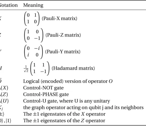
Qubit operators are represented by upper case Roman and Greek characters. For multi-partite states, the individual part being operated upon is indicated by a subscript. Thus, the expressionOiMj denotes the operatorsO andM acting on thei andj parts of the

state, respectively. Some of the more commonly used operators are listed below. Table 1.1– Notation for common qubit operators

Notation Meaning

X

0 1 1 0

(Pauli-X matrix)

Z

1 0

0 −1

(Pauli-Z matrix)

Y

0 −i i 0

(Pauli-Y matrix)

H p1

2

1 1

1 −1

(Hadamard matrix)

O Logical (encoded) version of operatorO

Λ(X) Control-NOT gate Λ(Z) Control-PHASE gate

Λ(U) Control-U gate, where U is any unitary

Kj the graph operator acting on qubit j and its neighbors

(18)

Chapter 2 Measurement Based Quantum

Computing

2.1 Introduction

In this chapter, we will describe a scheme for fault tolerant measurement based quan-tum computation. The scheme is implemented on a translation invariant qubit lattice using only single qubit measurements. In Chapter 3 we will see that this scheme has a very high error threshold of∼7.8×10−3_.

In this section, we introduce measurement based quantum computation in general, and in the next, we describe our specific proposal to make measurement based quan-tum computation fault tolerant. In Section 2.3, there is a brief note on how to implement the scheme in two physical dimensions. In the final section, we present an overview of the proposed scheme. It may be a good idea to read this first and keep it in mind as you read the rest of the chapter.

2.1.1 Computation as correlation

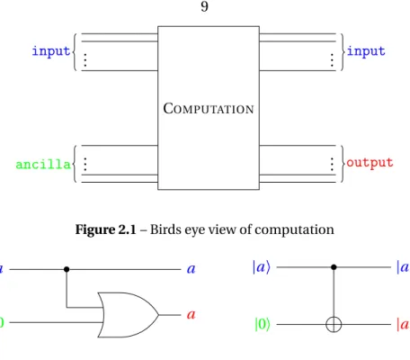
Normally, we think of computation as a process that takes some input, does some pro-cessing using the input, and outputs some results. Typically, the input consists of the actual input data as well as some ancillary bits that are “erased,” that is, set to some standard state. Once the computation completes, the output is stored in the ancillary bits. Ideally, at the end of the computation, the input bits have not been disturbed. This is represented schematically in Figure 2.1.

(19)

func-COMPUTATION

.. .

input

ancilla

.. .

input

output

Figure 2.1– Birds eye view of computation

a a

0 a

|a〉 |a〉

|0〉 |a〉

Figure 2.2– The COPY operation using classical and quantum circuits. In the quantum circuit, the output qubit has to be measured in the computational basis to get the value of thea bit.

tion on the input bits is defined by the pattern of gates in the circuit. In other models of computation the function may be defined differently. For example, in theTuring model, the function being computed is encoded as a sequence of instructions that have to be followed by theTuring machine.

Here, we are interested in the measurement based model of quantum computing. In this model, the correlation function is described by a sequence of measurements on individual qubits.

2.1.2 Measurement Based Quantum Computation

When a part of an entangled quantum system is measured, the state of the unmeasured portion depends on the initial state of the whole system, as well as the basis chosen for measurement (it also depends on the random measurement outcome, but this can be compensated for). Since a computer works by manipulating the state of bits, we can exploit this property of measurement to design a “measurement based quantum com-puter.” Such a computer consists of two parts; a pre-entangled “resource” state that starts out in some standard, highly entangled state, and a measurement pattern. The measurement pattern describes the algorithm (circuit) being implemented. In order to make our computer as simple to implement as possible, we would like to restrict our-selves to “local measurements,” i.e., to the measurement of only individual qubits.

(20)

Aside 2.1:

The Stabilizer Formalism

The stabilizer formalism [Dan97]can be used to represent multi-qubit states in terms of the operators under which they are invariant. Since the description of the space of such operators is exponentially smaller than the description of the space of states they represent, the stabilizer formalism is a powerful tool for analyzing such spaces.

An operatorK stabilizesa subspaceS, when∀ |ψ〉 ∈ S,

K|ψ〉=ψ.

The stabilizer formalism is particularly useful when the space of operators considered is a Hermitian subset of the Pauli group.

Given a subspace of states, if a unique group of stabilizer operators can be found that stabilize the subspace such that there is no state outside the subspace that is stabilized by the group, then the group is known as thestabilizer of the subspace. The stabilizer group can be represented fully by its generators (G). For a N element stabilizer, the generator has log₂Nelements, yielding a compact description of the stabilizer group.

The action of unitaries in the stabilizer formalism can be easily represented by noting thatU K U†_stabilizes_U_|_ψ_〉_,

U K U†U|ψ〉=U K|ψ〉=U|ψ〉.

Thus, the action of unitaryUon|ψ〉is equivalent to the action ofU·U†_{on the generators}

G.

Measurement in the Pauli basis can also be treated easily in the stabilizer formalism. Pauli measurements map stabilizers to new stabilizers. The effect of the measurement of Pauli operatorPon the stabilizer generatorG can be calculated as follows:

• IfPcommutes with all generatorsg ∈ G, the stabilizer is unchanged.

• SupposePanti-commutes with the generatorsg1, . . . ,gr. Then, the new generator

set G0 _{is obtained by replacing} _g

1 by c P and g2, . . . ,gr by g1g2, . . . ,g1gr, where c=±1 is the measurement outcome.

It can be easily checked thatG0_{generates the stabilizer of the post-measurement state.}

Example: Consider the Bell state|φ〉= p1

2(|00〉+|11〉). It has the stabilizer generator

G =〈X1X2,Z1Z2〉. Suppose we apply the Hadamard operator (H) to the first qubit, then

the new generator isG0 ₌_〈_X

1Z2, Z1X2〉. If we now measure theX1X2 operator on our

transformed state, we get a new generatorG00₌_〈_{c X}

1X2, Y1Y2〉.

(21)

X Z

Z

Z Z

1 2

4 3 0

Figure 2.3– a)The 2Dcluster state consists of qubits at the vertices of a two dimensional grid. It is the+1 eigenstate of theKj =Xj

Q

iZi operators, one at each vertex. It can be

created by starting with qubits in the|+〉state and performingΛ(Z)gates along the

edges of the lattice. b) A single qubit embedded in a larger cluster. The cluster is one example of a graph of degree four.

with their neighbors. The cluster state is an example of agraph state(see Aside 2.2) of degree 4. See Figure 2.3 for a schematic visualization of a 2D cluster state. The clus-ter state can be constructed by starting with all qubits in the|+〉state and performing a Λ(Z)gate along every edge in the cluster. TheΛ(Z)gates all commute, so their order is unimportant.

For the purpose of performing measurement based quantum computing alone, a 2D

graph state while sufficient, is not necessary. A simpler state could be used. Its choice is dictated by the fact that it is highly regular and easy to create experimentally, in a single time step, for example, in an optical lattice[Mar+02b; Mar+02a; Man+03a; Man+03b].

Let’s look at the effects of measuring qubits in cluster states. Since we want to keep things simple for the sake of experimental implementation, we will only consider only single qubit measurements.

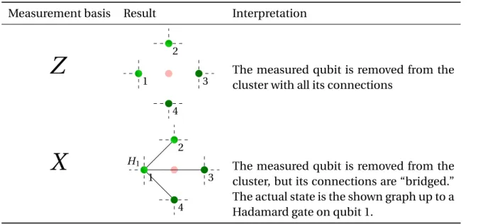
Measurement in the Pauli basis. Since the cluster state in Figure 2.3a is a graph state with stabilizer{Kj}Nj=1, we can use the stabilizer formalism (see Aside 2.1) to easily

de-duce the effect of measuring qubit 0 (from Figure 2.3b) in the Pauli basis. In particular, the measurement in theX andZ bases has a nice interpretation, shown in Table 2.1.

Measurement in a rotated basis. Measuring cluster qubits in a rotated basis allows us to create arbitrary correlations between input and output qubits. Recall that a cluster state is created by performingΛ(Z)gates between qubits prepared in the|+〉state. Now consider a slightly modified two qubit cluster state, in which the first qubit starts out in the state|ψ〉=α|0〉+β|1〉. The cluster state is then,

(2.1) _p1

2(α|0〉 |+〉+β|1〉 |−〉).

Now suppose that the first qubit is measured in the rotated basis p1

2{|0〉 ±e

iφ_|₁_〉}_{. The}

(22)

measure-Table 2.1– Measuring a cluster qubit in the Pauli basis

Measurement basis Result Interpretation

Z

1 2

3

4

The measured qubit is removed from the cluster with all its connections

X

1 2

3

4

H1 _{The measured qubit is removed from the}

cluster, but its connections are “bridged.” The actual state is the shown graph up to a Hadamard gate on qubit 1.

ment leaves the second qubit in the state

(2.2) α|+〉+ (−1)meiφβ|−〉=XmHUz φ|ψ〉.

Here,Uz(φ) =exp(iφZ)is a rotation about thez-axis of the Bloch sphere. We see that

the second qubit is left in a state equal to the first qubit, but rotated by the angle φ about thez-axis. In other words, the state of the second (output) qubit is correlated to the state of the first (input) qubit. Note that the angle of rotationφis set by the choice of measurement basis. However, because of the randomness of quantum measurement, we are left with an extra factor ofXm_{, that depends on the measurement outcome,} _m_.

These extra factors, called by-product operators are an unavoidable side effect of trying to perform gates by measurement, and have to be compensated for when performing measurement based computation. Fortunately, as we will see, this is not difficult.

Performing arbitrary single qubit gates. By chaining measurements in different ro-tated bases, it becomes possible to implement arbitrary single qubit gates by measure-ments alone. Consider the following sequence of qubits each measured in a different rotated basis

φ1 φ2 φ3 output

Using Eq. (2.2) we see that this sequence of measurements performs the following unitary on the output qubit

(2.3) U=HZm3_U

(23)

Wherem1,2,3are the three measurement outcomes. Using the identities

HZ H=X

(2.4)

HUz φH=Ux φ XUz φ=Uz −φX ZUx φ=Ux −φZ,

we can rewriteU as,

(2.5) U=Xm3_Zm2_Xm1_HU

z γUx βUz(α).

Whereα=φ1, β = (−1)m1φ2, γ= (−1)m2φ3. First note that this expression has exactly

the same form as Eq. (2.2). It is a rotation followed by a by-product operator that de-pends on the measurement outcomes. Thanks to Euler’s rotation theorem, we know that an arbitrary 3Drotation can be decomposed as a rotation about thez-axis, followed by a rotation about thex-axis followed by another rotation about thez-axis. Thus,U is an arbitrary single qubit unitary operator. Note that the choice ofφ2, φ3depends on the

measurement outcomes of measuring qubits 1 and 2 respectively. Thus, a time-ordering is imposed on our measurement pattern.

The by-product operators that remain at the end of the measurements are unimpor-tant. They need never be physically applied as they can always be accounted for when interpreting the measurement of the output qubits. For example, if the output qubit has to be measured in the computational basis, any extraZ by-product operators have no effect on the measurement outcome and anyX by-product operators simply flip the measurement outcome. When multiple single qubit operations are applied, all the by-product operators can be commuted through using Eq. (2.4) to appear on the left where they can be absorbed into the interpretation of the final measurement outcome.

Two qubit gates. While we now know how to perform arbitrary single qubit operations by measurement (and thereby create correlations between the input, and their corre-sponding output, qubits), we still need to be able to create correlations between differ-ent input qubits. This can be achieved by implemdiffer-enting a simple two qubit gate, the controlled-NOT(Λ(X))gate, defined, in the computational basis, as

(2.9) Λ(X)|c〉 |t〉=|c〉 |c+t mod 2〉.

AΛ(X)gate can be implemented by the construction shown below. Suppose qubits 1 and 4 were in the states|t〉and|c〉respectively, before the qubits were entangled. After the entangling operation, qubits 1 and 2 are measured in the X basis, leaving qubits 3 and 4 in the stateXm1+m2+1

3 Z

m1

4 |c+t mod 2〉 |c〉; wherem1,m2are the measurement

results. Thus, we have performed aΛ(X)between qubits 1 and 4, up to the by-product operatorXm1+m2+1

3 Z

m1

(24)

Aside 2.2:

Graph States

Graph states are a class of multiparticle entangled states that can be represented by mathematical graphs (collections of vertices connected by edges). The vertices repre-sent qubits, and the edges, entanglement between the qubits. AN qubit graph state|ψ〉 is defined as the state that obeys theN eigenequations

(2.6) Kj|ψ〉=|ψ〉; j =1 . . .N.

Where the operatorsKj are defined as

(2.7) Kj :=Xj

Y

i∈N(j)

Zi.

N(j) is the neighborhood of the j qubit, i.e., the neighborhood of the j vertex in the graph of the state. This is shown in the example below.

Z X

Z A graph state, showing

one stabilizer operator

Kj.

Bi-colorable graph states are a special class of graph states that we will encounter repeatedly. A bi-colorable graph is a graph whose vertices can be “colored” with two col-ors so that every vertex is connected only to vertices of a different color. Some examples:

An even cycle A 1Dcluster state An odd cycle. This isnot

bi-colorable.

Errors in a graph state. Graph states have the nice property that any error can be rep-resented in terms of chains ofZ operators. Recall that any single qubit operator can be expanded as sum in terms of Pauli operators and the identity. Now consider aX error on qubitj. It anti-commutes only with the stabilizer generators{Ki}, wherei runs over

the neighbors of j. Thus, it will affect only these operators. However, the error chain consisting ofZ operators acting on every neighbor of qubitj also anti-commutes with only these operators and thus is exactly equivalent to a singleXj error. This gives us the

identities,

(2.8) Xj =

O

i

Zi Yj =Zj

O

i

(25)

CNOT single qubit gate

network time

input

qubits

output

Figure 2.4– Schematic representation of a measurement based computer. Vertical arrows

represent measurement in theXbasis, dots represent measurement in theZ basis

and slanting arrows represent measurement in a rotated basis. Computation proceeds from left to right, with the output being obtained from the measurement results of the right most qubits. Each yellow stream represents the path of a “logical” qubit, as it moves from left to right. This computer operates on three logical qubits.

1 2 3 4

target in target out

control

With the CNOT gate and arbitrary single qubit unitaries, we have a universal set of gates and can perform any desired quantum computation[Bar+95]. We can combine these elements (single qubit operations andΛ(X)gates) into a full fledged measurement based quantum computer. For a schematic representation of a measurement based computer, see Figure 2.4.

While the quantum computer we have described will work very well in the absence of noise, in the real world, we must deal with noise and the impossibility of performing perfect quantum operations. Schematically, a measurement based computer works as follows:

• A 2Dcluster state is prepared

(26)

• The output is obtained by correctly interpreting the measurement results of the rightmost column, keeping in mind the by-product operators from previous mea-surements.

• Both the input data as well as the algorithm to be performed are encoded in the measurement pattern. We could instead have put the input data into the left most column of qubits before creating the cluster state, but encoding it in the measure-ment pattern gives us a consistent interpretation of a computer as something that takes classical data (a measurement pattern) as input and outputs classical data, in the form of measurement results, as well.

• We can think of the computer as operating on a register of “logical” qubits. At each time step (column), every logical qubit is represented by a single physical qubit. At the final time step the logical qubit is measured by measuring the physical qubit that encodes it.

The last item above points to a straightforward technique for making measurement based computers tolerant to noise. Rather than representing logical qubits by single physical qubits, we can instead encode a logical qubit into several physical qubits. How-ever, the naive approach of doing this directly, by using an error correcting code, such as the Steane code[Ste96], has certain drawbacks. The principal ones being that it will no longer be possible to implement the computation via single qubit measurements and creating a 2Dcluster state between logical qubits is much harder to do experimentally.

An alternative approach, described in[AL06], is to implement the fault tolerant ver-sion of the ideal circuit on the measurement based computer. Fault tolerance is thus achieved automatically, by the circuit construction itself. While this approach undoubt-edly works, it is abstract, and does not care what type of computer it is being imple-mented on. By using a fault tolerance scheme that directly leverages the architecture of the measurement based computation model, we can hopefully achieve better perfor-mance. Such a scheme is described in the next section. If you would like a more in depth treatment of the measurement based computation paradigm than presented above, see [DH06].

2.2 Fault Tolerant Measurement Based Quantum

Compu-tation

In the previous section, we saw that in the measurement based quantum computer, each logical qubit is represented by a single physical qubit at every timestep. In order to modify the measurement based computer to make itfault tolerant (see Aside 2.3), the first step is to use a quantum error correcting code to encode logical qubits. We must chose this code carefully to be compatible with the measurement based paradigm (i.e., an easy to prepare initial state with only single qubit operations to follow).

(27)

Aside 2.3:

Fault tolerance

In general terms, when we say that we want a computer to be fault tolerant, we mean that it should be somehow “resistant to noise.” In other words as long as the noise af-fecting the computation is somehow bounded, we should be able to design a computer that computes with arbitrary accuracy, without too much overhead.

This requirement is formalized in the context of quantum computation via the

Threshold Theorem.

Theorem 1. If the noise per elementary operation is below a constant non-zero threshold then an arbitrarily long quantum computation can be performed with arbitrary accuracy and small operational overhead.

This theorem has been proven for the circuit model of computation[AGP06]and it applies, as well, to the measurement based model, via the mapping in[AL06].

While the threshold theorem shows that there must exist an implementation of the computer that is fault tolerant, it is silent on how to construct one. In this chapter and the next, we present a design of a fault tolerant measurement based quantum computer that has a very high threshold and whose overhead requirements scale well with increas-ing circuit size.

a) b)

Figure 2.5– The cubic lattice used for fault tolerant measurement based computation. a) The

elementary cell of the lattice. It has 18 qubits and is tiled in 3Dto build the lattice.

The solid lines indicate entanglement between the qubits. The lattice is a

(28)

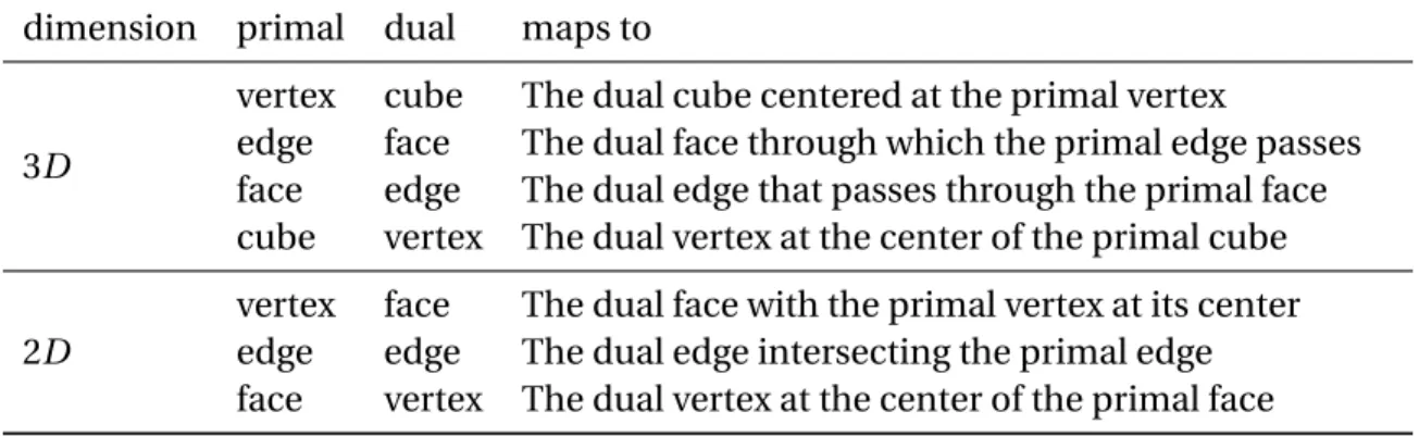
Table 2.2– The duality transforms in two and three dimensions. The transforms aresymmetric

((x∗₎∗₌_x₎_.

dimension primal dual maps to

3D

vertex cube The dual cube centered at the primal vertex

edge face The dual face through which the primal edge passes face edge The dual edge that passes through the primal face cube vertex The dual vertex at the center of the primal cube

2D

vertex face The dual face with the primal vertex at its center edge edge The dual edge intersecting the primal edge face vertex The dual vertex at the center of the primal face

along the other dimension, from left to right. Surface codes are two dimensional, so a measurement based computer with its qubits encoded in a surface code, will be three dimensional. The 3D structure we use is a cubic lattice(L) with qubits on the faces and edges of the elementary cell (see Figure 2.5). Hereafter, the computer based on this lattice will be referred to as theC3D.

If we define the elementary cell to have a side of length 2 units, then, we can identify two sub-lattices within the full lattice. Call these sublattices primal(Lp)and dual(Ld).

Each sub-lattice is a cubic lattice, but now only with qubits on its edges. The vertices of these lattices are located at the co-ordinates:

Lp= (e[v e n],e,e)

Ld = (o[d d],o,o).

Ld isdualtoLp under the symmetric mapping()∗, defined in Table 2.2.

The sub-lattices are important as all the structures we eventually introduce for quan-tum computation belong on one or the other of these sub-lattices, and the way they in-teract depends on which sub-lattice they belong to. Furthermore, throughout this work, we adopt the convention that logical qubits are encoded on the primal sub-lattice while the dual sub-lattice is used to encode correlations between the logical qubits. The oppo-site convention of using the dual lattice to encode logical qubits is also possible. Indeed, the two conventions can even be mixed to an extent. However, for the sake of clarity and standardization, we will stick to the first convention.

The first stage in definingC3D is to define the encoding of the logical qubits, which

we will address in the next section.

2.2.1 The Logical Qubit

In the measurement based computer (Figure 2.4), the computation could be divided into timesteps with each logical qubit being encoded into a single physical qubit at every time step. Similarly, for C3D, the computation can be divided into timesteps. At each

(29)

Aside 2.4:

Surface codes

Surface codes [SA98; Den+02a], are a way of encoding quantum information (states) into the topology of a lattice of qubits. The simplest (and most directly relevant) example is to use

a 2D lattice with the qubits living on the edges of the lattice. Such a state is a stabilizer state

(see Aside 2.1), with two types of stabilizer generators (plaquette and site). If all the stabilizers

are enforced, then the stabilized subspace consists of a single state, the+1 eigenstate of all the

stabilizers. By itself, this state is not very interesting, but if we relax one of the constraints (i.e.,

no longer require a particular generator to have eigenvalue+1), then the stabilized subspace

has dimension two. We can interpret the new state as carrying a localized excitation at the site

of the relaxed generator, or aquasi particle. In the diagram below, we see an example of such

quasi-particles, called “holes.”

Z Z

X X X X

plaquette operator site operator

Zchain

Xchain

“hole”

Z, X

In this diagram, we see the various structures defined on the lattice. First, the stabilizer genera-tors, of two types, plaquette and site. It is easy to see that they commute with each other. Errors

on the lattice can be eitherZ chains, orXchains. AXchain consists of theXoperator acting on

all edges that intersect the dashed blue line, whileZ chain consists ofZ operators acting along

the thick red line. Error chains anti-commute only with plaquette and site operators at their ends and thus leave syndrome only at their ends (syndrome consists of the results from measuring the plaquette and site operators at all locations on the lattice).

Encoding logical qubits. In the third diagram, we see an example of using a pair of quasi

particles to encode a logical qubit. The logicalZ operator is defined as any closed loop ofZ

operators that encircles one of the holes, while the logicalXoperator is defined as any chain ofX

operators stretching between the two holes. A similar set of definitions exists for a pair of holes made up of site operators.

Error correction. First note that any closed loop that does not enclose a hole is equivalent to

the logical identity operation, since it is in the stabilizer of the state and commutes with theX

andZ operators. Since error chains leave a syndrome only at their ends, we just have to match

(30)

y

network time t

x

code plane for surface code

3D cubic lattice

Figure 2.6– The schematicC3D. Logical qubits are encoded in the surface code on a 2Dplane.

At each timestep, the left most plane is measured, and the logical qubits move onto the next plane. The output is obtained when the rightmost plane is measured.

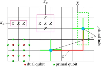
Z X Z Z Z

Z Z X

dual qubit primal qubit

Kd _pr

imal

hole

Kp _X

Z

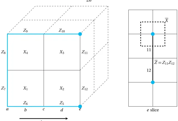
Figure 2.7– A 2Dslice ofLpshowing a logical qubit. The stabilizer generators of the full 3D

lattice when projected onto the slice are of two types,Kp andKd. The logicalX

operator consists ofXacting on every edge intersected by the dashed line.Z

consists of Z operators acting on all the edges marked by the thick red line.

the plane is measured, the logical qubits move onto the next plane, and so on, until they are finally measured on the output plane at the right. By correctly interpreting this measurement result (keeping in mind the results from measuring previous planes), we get the result of the computation. This idea is represented schematically in Figure 2.6.

Just as was the case for the surface code (Aside 2.4), logical qubits in the C3D are

made up of pairs of “holes.” By convention, the holes live on 2Dslices ofLp. We saw

in the case of the surface code that a hole introduces a degree of freedom, raising the dimension of the stabilized subspace from one to two. A hole has exactly the same effect here. Consider Figure 2.7, which shows a 2Dslice ofLp. The stabilizer generators of the

full 3Dlattice, when projected onto the slice, are of the formKp andKd. We can define a

site operator (analogous to the site operator of the traditional surface code in Aside 2.4), as shown in the figure. By relaxing the requirement that the plaquette operator have eigenvalue+1, we introduce a degree of freedom, or a hole.

(31)

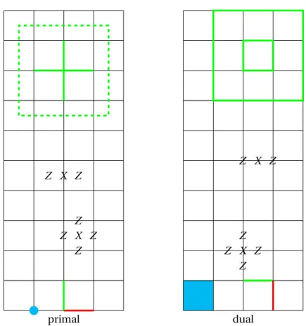
How-Z Z Z Z X X

Z Z

X

Z Z

X

Z Z

dual primal

Figure 2.8– The mapping from slice to surface code. See the discussion in the text.

ever, by measuring the face qubits in theX basis, we can convert the slice to a surface code. When the measurement pattern forLis described, we will see that the face qubits are indeed measured in theX basis. To understand the mapping from slice↔surface code, we consider the 2Dlattice dual to the slice (see Table 2.2 and Figure 2.8). The dual lattice has qubits on edges and vertices. TheKd stabilizers are associated with the edges

of the dual lattice and theKp stabilizers with the vertices. By multiplying fourKd

sta-bilizers, we get a plaquette operator consisting of theX operator acting on the edges of the plaquette. Each edge is shared by two faces, thus there are two edges per face and therefore twoKd operators per face. One of these can be replaced by the plaquette

op-erator. When the vertex qubits are measured inX, the otherKd is replaced by a single X operator, associated with the corresponding vertex. By multiplying this operator with

Kp we are left with a site operator consisting ofZ acting on the arms of the site. Thus,

the stabilizer after measurement consists of plaquette and site operators, just as for the surface code in Aside 2.4 (except that the roles of theX andZ operators are reversed). Since the dual lattice supports a surface code, the primal lattice also supports the dual of the same code.

A pair of primal holes supports a single qubit. The logicalX operator is a loop ofX

(32)

Table 2.3– Notation for the components of the sub-latticesLp,Ld

Feature Lp Ld

vertex v v =q∗

edge e e =f∗

face f f =e∗

cube q q=v∗

This is a property of the surface code, and is easy to check. Since the loop and chain must intersect in an odd number of edges, it is easy to see that[X,Z] =−1. Thus, by adding pairs of holes to the slice, we can encode as many logical qubits as needed.

Remember that a hole is really just a location on the lattice where the corresponding stabilizer is not enforced. In the context of a measurement based computer, where slices are measured destructively (rather than measuring stabilizers directly, individual qubits are measured and the value of the stabilizers is computed by combining the measure-ment results), this means that when interpreting the measuremeasure-ment results, the value of the missing stabilizers must not be computed. ForC3D, this is automatically ensured

by the construction of the lattice and the measurement pattern. What this means will become clear in the next section, where we define in detail the various components of C3D.

2.2.2 The Topology of It

In order to understand precisely how the computation proceeds inC3D, we will first have

to identify and define the various structures that make it up. We have already defined the cubic latticeL, along with the two sub-latticesLp,Ld that are dual to one another

(see Table 2.2).

The sub-latticesLp,Ld are made up of vertices, edges, faces and cubes. These will

be referred to by the notation defined in Table 2.3. The various components are related to each other, by theboundary operator (∂). The boundary of a cube is the set of six faces, the boundary of a face is the set of four edges and the boundary of an edge is two vertices.

Intuitively, the boundary operator is quite clear. For example the boundary of four adjacent faces would be the eight edges on the “outside” of the faces. However, the boundary operator is really a topological operator and to make its definition precise, we need to set up achain complex [All02]on L. This is done in Aside 2.5. With the precise definitions out of the way, we can enumerate the various objects that live inC₃D.

Qubits. Qubits inL come in two flavors, primal or dual. Primal qubits are located on edges ofLp or conversely, faces ofLd. Dual qubits are located on the edges ofLd or

(33)

X X X

Z Z

Z

Z Z

Z

Z Z

=X

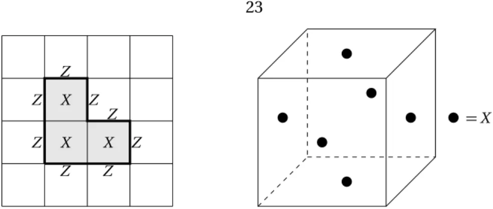
Figure 2.9– Examples of correlation operators. On the left is a correlation operator in 2DwithX

acting on the faces andZon the boundary. On the right is a special type of

correlation operator, the syndrome operator. It consists ofXacting on the six faces

of a cube.

Correlations. A correlation is defined as a collection of faces, or formally, a 2-chainc2

(see Aside 2.5). It is not strictly necessary for a correlation to be made up of contiguous faces, but all the correlations we will encounter in this work will be contiguous. Associ-ated with every correlationc2, is acorrelation operator, defined as

(2.10) K(c2):=

O

f∈c2

X f

Z ∂ f .

In words, a correlation operator consists of theX operator acting on the face qubits and theZ operator acting on the qubits in the edges that form the boundary of the faces. Correlations can be either primal or dual. A primal correlation has X acting on dual qubits, withZ acting on primal qubits, while a dual correlation is the converse. Some examples are in Figure 2.9.

Correlations are used to move logical qubits forward with time and also to mediate interactions between logical qubits.

Errors. Recall in Aside 2.2, we saw that for a graph state, any error can be represented as a chain ofZ operators. So it is natural to define errors as sets of edges. The edges need not be connected. Formally, an error is a 1-chain c1 (see Aside 2.5). Associated

with every error is anerror operator, defined as

(2.11) E(c1):=

O

e∈c1

Z(e).

In words, an error operators consists of theZ operator acting on the qubits in a set of edges. Errors can also be either primal or dual. A primal error operator isZ acting on primal qubits, while a dual error operator isZ acting on dual qubits.

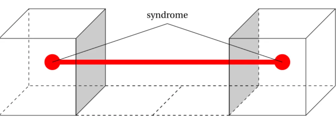
Syndrome. Syndrome is extracted from the measurement results. It is used to detect the presence and type of errors that are affecting the computation. In the case ofC3D

(34)

syndrome

Figure 2.10– Error chains leave syndrome at their ends.

Recall from Table 2.2 that every vertex is dual to a cube. This tells us what the operator that has to be measured to yield the syndrome at a vertex should be. It is the correlation associated with the faces of the cube dual to that vertex. Thesyndrome operatoris

(2.12) S(v):= O

f∈∂v∗

X(f).

This follows from Eq. (2.10) and the observation that∂2_q₌_{0 (see Aside 2.5). In words, a}

syndrome operator is theX operator acting on the six faces of a cube. See Figure 2.9 for an example. Note that when restricted to a 2Dslice, the syndrome operator becomes a site operator, as expected.

Syndrome and errors. Primal syndrome detects primal error chains while dual syn-drome detects dual error chains. Letc1be an error chain,q be a dual cube

correspond-ing to primal vertex v = (q)∗_{. The error operator} _E(_c₁) _{anti-commutes with the} syn-drome operatorS(v)only if v ∈∂c1. Thus, error chains show syndrome only at their

ends, just as for the surface code. This is shown in Figure 2.10.

Correlations and errors. Primal correlations are affected by dual error chains and dual correlations are affected by primal error chains. This is easy to see when you remember that error operators are made up ofZ operators on edges, while correlation operators haveX acting on face qubits. A primal correlation hasX acting on primal faces, which are also dual edges. Thus, only a dual error operator can anti-commute with a primal correlation operator.

Furthermore, an error chain will only affect a correlation if it intersects the corre-lation an odd number of times. This follows from the the observation, E(c1)K(c2) =

(−1)|{c1}∩{c2∗}|K(c

2)E(c1). If the number of intersections,|{c1} ∩ {c2∗}|, is odd, the

correla-tion is conjugated to−K(c2)by the error, otherwise it is left unchanged.

(35)

Aside 2.5:

Homology on

_L

Define the chain groups as follows (wherezk∈Z2)

object Chain group Basis

vertices C0={c0:c0=

P

kzkvk} B(C0):={vk : vertices inLp}

edges C1={c1:c1=

P

kzkek} B(C1):={ek: edges inLp}

faces C2={c2:c2=

P

kzkfk} B(C2):={fk: faces inLp}

cubes C3={c3:c3=

P

kzkqk} B(C3):={qk : cubes inLp}

The groups{Ci}3_i₌₀are Abelian under componentwise addition. For example,c1+c₁0 =

P

kzkek+

P

kzk0ek =

P

k(zk+z0k)ek. For eachi =1 . . . 3, there exists a homomorphism

∂i mappingCi toCi−1, with the composition∂i−1◦∂i =0. With these definitions,

C :={C0,C1,C2,C3},

is a chain complex [All02]and∂ is a boundary operator that maps the chainci to its

boundary which is a chainci−i. Similarly, the dual chain complex,C∗:={C₀∗,C₁∗,C₂∗,C₃∗}

can be defined onLd.

We are now ready to define homology. Two chainscn,c_n0 ∈Cn are said to be

homo-logically equivalent if there exists somecn+1∈Cn+1, such thatc_n0 =cn+1+∂cn+1. In other

words,c0

n =hcn if they differ by the boundary of a chain of the next higher dimension.

The concept of homology encapsulates the property of surface codes that an error chain has syndrome only at its end-points (i.e., only at its boundary), and that we can correct such a chain by applying any chain that has the same end points.

Of particular interest to us, is the concept of relative homology. Suppose a chain complex is defined on a spaceX and there exists a sub-spaceD ⊂ X. Two chains are equal w.r.t relative homology, c0

n =r cn, if there exists some cn+1 ∈Cn+1(X) and dn ∈ Cn(D)such thatc_n0 =cn+∂cn+1+dn. This formalizes the idea that in a surface code, an

error chain can start and end on a pair of defects (holes), and that the effect of the chain on the logical qubit is the same irrespective of the actual shape of the chain.

become clear as we progress. Formally, a defectd is defined as a connected set of edges and the faces they “contain,”

(2.13) d :={e :e ∈d} ∪

f :{∂f} ∩d={∂f} .

In words, a defect is a set of edges alongwith the faces the set of edges contains. A face is contained by a set of edges if its boundary is in the set of edges. Defects are either primal or dual, depending on whether they contain primal or dual edges and faces.

(36)

The measurement pattern. SinceC3D follows the measurement based quantum

com-puter paradigm, all measurements are single qubit measurements. The basis in which a particular qubit is measured depends on what part ofC3D it belongs to. The different

parts that have different measurement patterns are listed below.

• Singular qubits. These qubits are measured in a basis rotated about thez-axis |0〉+exp(iφ)|1〉

. The value ofφdepends on the type of ancilla we are trying to create with the singular qubit.

• Defect qubits. Recall that defects are made up of two types of qubits, edge qubits and face qubits. Edge qubits are measured in theZ basis, while face qubits are measured in theX basis. This is true for both primal and dual defects.

• Bulk qubits. All the remaining qubits are measured in theX basis.

Now that we have specified the measurement pattern, we can see how it interacts with the surface code on a 2D slice ofLp. Recall that “holes” on the surface code are

simply locations where the corresponding site operator is not enforced. A hole is really the projection of a defect that extends in the time direction onto the slice. Therefore, the edges ofLp that extend in the time direction from the vertex at which a hole is

lo-cated are defect edges. But primal edges are dual faces, so these two edges are also two faces of a dual cube centered at the vertex. Normally, the syndrome associated with the vertex would have been obtained by measuring the six faces of the dual cube in theX

basis. Now however, because two of the faces are defect edges and therefore measured in theZ basis, the syndrome bit associated with the vertex is lost, and thus the stabilizer associated with it is not enforced. Note that sinceL is a graph state and all errors on it areZ chains, the plaquette operators of the surface code (that consist ofZ acting on the edges of a plaquette) are automatically enforced. The site operators are enforced using the syndrome obtained from the measurement of the dual cubes centered at each primal vertex.

Correlations and defects. In a primal defect, edges in the boundary of a primal 2-chain are measured in theZ basis. Recall that a primal correlation consists of X operators on primal face (dual edge) qubits andZ operators on primal edge qubits. Therefore, a primal correlation can “end on” a primal defect. By “end on,” we mean that it can have a primal defect as its boundary. Similarly, dual correlations can only end on dual defects. Similarly, primal correlations can wrap around dual defects and dual correlations can wrap around primal defects. This is analogous to having chains encircling holes in the surface code. In this manner, defects can be used to “guide” correlation surfaces.

(37)

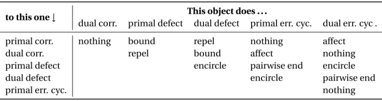
Table 2.4– Relationships between correlations, syndrome, defects and errors. “AboundsB” is

synonymous with “Bends inA.” The displayed objects do not interact with

themselves. The relations are symmetric.

to this one↓ This object does . . .

dual corr. primal defect dual defect primal err. cyc. dual err. cyc .

primal corr. nothing bound repel nothing affect

dual corr. repel bound affect nothing

primal defect encircle pairwise end encircle

dual defect encircle pairwise end

primal err. cyc. nothing

However, for each defectd, there will be one syndrome bit associated with the defect as a whole. This is because there is a correlation surface (2-chain) that wraps around the defect as a whole. Since it wraps around the defect, it is closed, has no boundary and is of the formN

iXi. When the qubits in the bulk region are measured in theX basis, this

correlation yields an extra syndrome bit.

Errors and defects. A primal error chain can end in a primal defect. This is because, primal syndrome is lost at a primal defect, as discussed above. Similarly, dual error chains can end in dual defects. However, there is a syndrome bit associated with the defect as a whole and this detects an error chain ending in the defect if the number of intersection between the correlation surface and the chain is odd. Thus error chains can

pairwiseend in defects.

The relationships between correlations, syndrome, defects and errors is summarized in Table 2.4.

2.2.3 Initialization and Measurement of Logical Qubits

The first step in performing a computation is preparing logical qubits in a known state. In the following discussion, the preparation and measurement of states in theX,Z bases is shown using defects made up of single edges. This is for clarity and ease of presen-tation. In an actual fault tolerant construction, the defects would be thick, as will be explained subsequently. The initialization in the rotated states however, requires the use of single qubits and cannot be topologically protected. These logical qubits must therefore be distilled before being used. The distillation will also be discussed later.

Initialization in an eigenstate ofZ. In order to create a logical qubit that is in an eigen-state of theZ operator, we use the construction shown in Figure 2.11. The qubits on the blue edges are measured in theZ basis, while all other qubits are measured in theX

Using Graph States for Quantum Computation and Communication

Communication

Kovid Goyal

Acknowledgements

Abstract

Contents

List of Figures

List of Tables

List of Asides

Chapter 1

Introduction

1.1

Computation Powered By Quantum Mechanics

1.1.1

A Working Quantum Computer?

1.1.2

Measurement Based Quantum Computation

1.1.3

Topological Error Correcting Codes

1.2

Quantum Mechanics in Communication

1.3

Structure

1.4

Notation

Chapter 2

Measurement Based Quantum

Computing

2.1

Introduction

2.1.1

Computation as correlation

2.1.2

Measurement Based Quantum Computation

Aside 2.1:

The Stabilizer Formalism

Z

X

Aside 2.2:

Graph States

network time

2.2

Fault Tolerant Measurement Based Quantum

Compu-tation

Aside 2.3:

Fault tolerance

2.2.1

The Logical Qubit

Aside 2.4:

Surface codes

2.2.2

The Topology of It

Aside 2.5:

Homology on

L

2.2.3

Initialization and Measurement of Logical Qubits

_L