DOI: 10.1515/tmmp-2017-0014 Tatra Mt. Math. Publ.69(2017), 61–73
MULTIDIMENSIONAL COPULA MODELS
FOR PARALLEL DEVELOPMENT
OF THE US BOND MARKET INDICES
Jozef Komorn´ık — Magdal´ena Komorn´ıkov´a – – Tom´aˇs Bacig´al — Cuong Nguyen
ABSTRACT. Stock and bond markets co–movements have been studied by many researchers. The object of our investigation is the development of three U.S. in-vestment grade corporate bond indices. We concluded that the optimal 3D as well as partial pairwise 2D models are in the Student class with 2 degrees of freedom (and thus very heavy tails) and exhibit very high values of tail dependence coef-ficients. Hence the considered bond indices do not represent suitable components of a well-diversified investment portfolio. On the other hand, they could make good candidates for underlying assets of derivative instruments.
1. Introduction
In this paper, we apply 2- and 3-dimensional copula models to the triple of time series of returns of indices of US financial markets (using daily data from Bloomberg). The triple of indices (US CBI) contains the Bank of America Merrill Lynch US Corporate Bond Index (ML), the Barclays US Corporate & Investment Grade Index (BAR), Dow Jones Corporate Bond Index (DJ) from the time period from January 1997 to May 2014. Our results show high values of Kendalls correlation coefficients as well as tail dependencies between all couples of this triple of indices.
The paper is organized as follows. The second section is devoted to a brief over-view of the theory of copulas. In the third section we present the utilized method-ology of copula fitting to two- and three-dimensional time series. The fourth section contains application to real data modeling. Finally, some conclusions are presented.
c
2017 Mathematical Institute, Slovak Academy of Sciences.
2010 M a t h e m a t i c s S u b j e c t C l a s s i f i c a t i o n: 62H20, 62H86, 62P20, 91G70.
K e y w o r d s: bond market indices, Copulas, Cramer-von Mises test statistics, GoF test, Vuong and Clarke tests.
2. Copulas
Copula represents a multivariate distribution that captures the dependence structure among random variables. It is a great tool for building flexible multi-variate stochastic models. Copula offers the choice of an appropriate model for the dependence between random variables independently from the selection of marginal distributions. This concept was introduced in the late 50’s and became popular in several fields beyond statistics and probability theory, such as finance, actuarial science, fuzzy set theory, hydrology, civil engineering, etc.
Due to [11]
F(x1, . . . , xn) =CF1(x1), . . . , Fn(xn),
whereF is joint cumulative distribution function of random vector (X1, . . . , Xn),
Fi, i = 1, . . . , n is marginal cumulative distribution function of Xi, and C : [0,1]n → [0,1] is a copula which is n-increasing function with 1 as neutral element and 0 as annihilator, see, e.g., [8].
Besides three fundamental copulas
M(x1, . . . , xn) = min{x1, . . . , xn}, W(x1, x2) = max{x1+x2−1,0},
Π(x1, . . . , xn) =
n
i=1
xi
which model perfect positive dependence, perfect negative dependence (not ap-plicable for n >2) and independence, respectively, there exist numerous para-metric classes, such as Archimedean, Extreme-Value and elliptical copulas. With-in the last there belong such important parametric families as Gaussian copulas
CG(x1, . . . , xn) = ΦΦ−11(x1), . . . ,Φ−n1(xn)
(1)
and Student t-copulas
Ct(x1, . . . , xn) =tt1−1(x1), . . . , t−n1(xn)
(2)
(where Φ and tare joint distribution functions of multivariate normal and Stu-dent t distributions, similarly Φ−i 1 and t−i1 are univariate quantile functions related toXi), able to flexibly describe dependence in multidimensional random vector.
The Archimedean class [5]
CA(x1, . . . , xn) =φ(−1)φ(x1) +· · ·+φ(xn) (3)
Tail dependencies are functions that describe the dependence structure of multi-dimensional distributions in the tail and are defined (for bivariate case) as follows [8].
LetX1 and X2 be continuous random variables with distributions functions
F1 and F2 and with copula C, then the lower tail dependence coefficient is defined by
λL= lim
u→0+P r
X1≤F1−1(u)|X2≤F2−1(u)
= lim
u→0+
C(u, u)
u , (4)
and the upper tail dependence coefficient by
λU= lim
u→1−P r
X1 > F1−1(u)|X2 > F2−1(u)
= lim
u→1−
1−2u+C(u, u)
1−u . (5)
(provided that the above limits exist).
Note that in the above formulas (4) and (5), the role of X1 and X2 are exchangeable.
Analogically for an-dimensional copulaC(x1, . . . , xn) we define [3]
λL,i= lim
u→0+P r
Xi ≤Fi−1(u)|Fj−1(u)≤u for allj =i (6) and
λU,i= lim
u→1−P r
Xi ≥Fi−1(u)|Fj−1(u)≥u for allj=i. (7)
Since the role of the variables for Archimedean copulas is exchangeable, the above formulas (6) and (7) ofλL,i and λU,i do not depend oni for them.
Archimedean copulas can capture different tail dependencies, i.e., λL =λU. However, their exchangeability property can cause problems for their utilization for modeling data in higher dimensions. The Gaussian copulas do not have lower and upper tail dependencies. Thet copula has upper tail dependenciesλU,i (and because of radial symmetry) equal lower tail dependenceλL,ifori= 1, . . . , n.
3. Fitting of copulas
Given m observations {Xj,i}i=1,...,m of j-th random variable Xj, the param-eters θ of all copulas under consideration were estimated by maximizing the likelihood function
L(θ) =
m
i=1
cθ(U1,i, U2,i, U3,i), (8)
wherecθ denotes density of a parametric copula familyCθ, and
Uj,i= 1
m+ 1
m
k=1
are so-called pseudo-observations. Goodness-of-fit was performed by a test pro-posed by [6] and based on empirical copula process using Cramer-von Misses test statistic SCM = m i=1
Cθ(U1,i, U2,i, U3,i)−Cm(U1,i, U2,i, U3,i)2 (10)
with empirical copula
Cm(x) = 1
m m i=1 3 j=1
1(Xj,i≤xj)
and indicator function1(A) = 1 wheneverAis true, otherwise1(A) = 0. For selection of the optimal copula for a given couple, we utilized the scoring criteria based on Vuong and Clarke Tests [1].
The test proposed by C l a r k e (2007) [2] allows to compare non-nested mod-els with copulas having densities c1 and c2 with estimated parameter sets θ1 and θ2. The null hypothesis of statistical indistinguishability of the two mod-els is
H0:P r(ki >0) = 0.5 for all i= 1, . . . , m, (11) where
ki = log
c1(ui|θ1)
c2(ui|θ2) for observations ui, i= 1, . . . , m.
Since under statistical equivalence of the two models the log likelihood ratios of the single observations are uniformly distributed around zero and in expecta-tion 50% of the log likelihood ratios greater than zero, the test statistic
B=
m
i=1
1(0≤ki ≤ ∞), (12)
where1is the indicator function, has the binomial distribution with parameters m andp= 0.5.Model 1 is interpreted as statistically equivalent tomodel 2 ifB is not significantly different from the expected valuem p=m/2.
The likelihood-ratio based test proposed by V u o n g (1989) [12] can be used for comparing non-nested models. For this letc1andc2be two densities of copu-las with estimated parameter setsθ1 andθ2. We then compute the standardized sumν of the log differences of their pointwise likelihoods
ki = log
c1(ui|θ1)
c2(ui|θ2) for observations ui∈[0,1], i= 1, . . . , m, i.e., statistic
ν= 1
m
m
i=1ki
m
i=1(ki−¯k)2
with k¯= 1
m m
i=1
V u o n g (1989) [12] shows thatνis asymptotically standard normal. According to the null-hypothesis
H0: E[ki] = 0 for all i= 1, . . . , m, (14)
we hence prefer model 1 to model 2 at levelαif
ν > Φ−1(1−α/2),
where Φ−1 denotes the inverse of the standard normal distribution function. If
ν <−Φ−1(1−α/2),
we choosemodel 2. If, however,
|ν| ≤ Φ−1(1−α/2),
no decision among the models is possible.
4. Modeling results
All calculations were done in R [9] with the help of packages [7] and [10]. In package [10] several bivariate copula families are included for bivariate analysis as well as for multivariate analysis. It provides elliptical (Gaussian and Student-t) as well as Archimedean (Clayton, Gumbel, Frank, Joe,BB1, BB6, BB7
and BB8) copulas. For any copula families rotated versions
C90(x1, x2) =x2−C(1−x1, x2),
C180(x1, x2) =x1+x2−1 +C(1−x1,1−x2) survival copula,
C270(x1, x2) =x1−C(x1,1−x2),
are included to cover negative dependence, too. For more and detailed informa-tion about copula families see [8].
The Vuong as well as the Clarke test compare two models against each other allow for a decision among several models. In B e l g o r o d s k i [1] this is used for bivariate copula selection. It compares amodel 0 to all other possible models under consideration. If model 0 is favored over another model, a score of +1 is assigned and similarly a score of -1 if the other model is determined to be superior. No score is assigned, if the respective test cannot discriminate between two models.
We can see the graphs of considered triple of time series in the Figure 1. We see that the Merrill LynchUSCorporate Bond Index(ML)mostly leads the remaining two in the considered triple (with deeper losses in the crisis period).
Figure 1. US Corporate Bond indices.
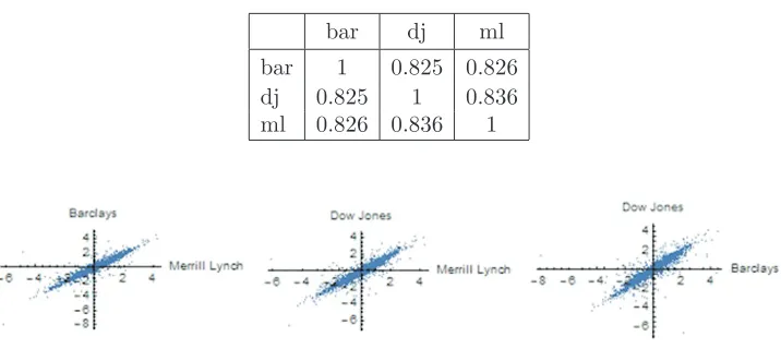
Before further analyses, we filtered all considered time series by ARMA --GARCHfilters [4]. Results of the introductory standard analysis of the residuals are presented in Table 1 and Figure 2. We see that the values of the Kendall’s correlation coefficients are fairly high (contained in the interval [0.825, 0.836]) for all 3 considered couples of residuals. Their strong dependencies are illustrated in Figure 2.
Table 1. Values of the Kendall’s correlation coefficient for all couples of
the (filtered) returns of US CBI.
bar dj ml
bar 1 0.825 0.826
dj 0.825 1 0.836
ml 0.826 0.836 1
We prolonged our analyses by examining developments of the Kendalls corre-lations. We have chosen annuals frequency of calculations of Kendalls correlation coefficients over the intervals of 24 months overlapping by 12 months with the intervals for calculation of the neighboring values of Kendalls correlation coef-ficient. Altogether, we have calculated a sequence of 17 such values. The last of them was calculated from the interval of 17 months. We can see (Figure 3) that all three correlation coefficients exhibit extremely parallel development and their values are contained in the interval [0.7, 0.95] of high values and by far do not approach the rejection limits for tests of their zero value (that equals 0.029).
Figure 3. Evolution of Kendall’sτ for all couples of the (filtered) returns of US CBI.
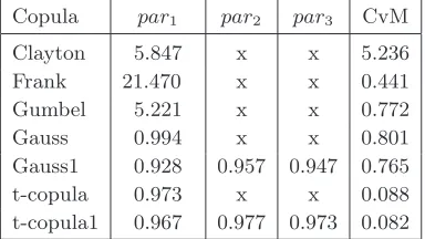
Table 2. GoF test for 3D copulas, based on the Cramer–von–Mises method.
Copula par1 par2 par3 CvM Clayton 5.847 x x 5.236 Frank 21.470 x x 0.441 Gumbel 5.221 x x 0.772 Gauss 0.994 x x 0.801 Gauss1 0.928 0.957 0.947 0.765 t-copula 0.973 x x 0.088 t-copula1 0.967 0.977 0.973 0.082
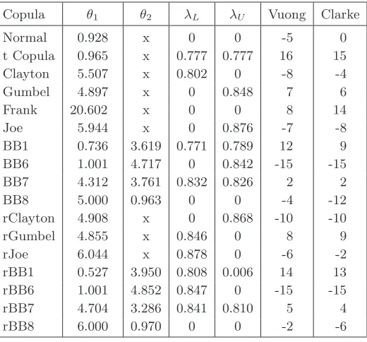
(that have very similar values) is closely followed by the best one-parameter Student class model (with the parameter that is also close to the mentioned 3 parameters of the best 3-parametric model). The best copula with respect to Cramer–von–Mises (CvM) test statistic is the trivariate t-copula with test statistic SCM = 0.082 and parameters: and The best one–parameter Student class copula (with Cramer–von–Mises test statistic SCM = 0.088) has parame-ters: ρ = 0.973, λL = λU = 0.804 and degrees of freedom df = 2. A very low value of the degree of freedom indicate heavy tails that also correspond to fairly high values of the coefficients of tail dependence. Among the bivariate copula models the best ranking according to the Vuong test was achieved (for all three considered couples) by the models in the Student class quite closely followed by the models in the BB1180 class. According to the scoring based on the Clarke test, the results are slightly different. The models from the Student class are the best for the couple bar & dj and dj & ml, while they share the best rating with the BB1180 for the couple bar & ml (see Table 3, Table 4 and Table 5). The optimal bivariate Student class copulas have 2 degrees of freedom for all three couples. Their contour plots are presented in Figure 4.
Table 3. Results for Vuong–Clarke scoring test for couple bar & dj.
Copula θ1 θ2 λL λU Vuong Clarke
Figure 4. Contour plot of densities of t-copulas for couples bar & dj (left),
bar & ml (middle) and dj & ml (right).
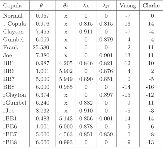
Table 4. Results for Vuong–Clarke scoring test for couple bar & ml.
Copula θ1 θ2 λL λU Vuong Clarke
Normal 0.957 x 0 0 -7 0 t Copula 0.976 x 0.815 0.815 16 14 Clayton 7.455 x 0.911 0 -7 -4 Gumbel 6.069 x 0 0.879 4 4 Frank 25.580 x 0 0 2 11 Joe 7.380 x 0 0.901 -13 -11 BB1 0.987 4.205 0.846 0.821 12 10 BB6 1.001 5.902 0 0.876 4 2 BB7 5.000 5.949 0.890 0.851 0 -5 BB8 6.000 0.985 0 0 -14 -16 rClayton 6.374 x 0 0.897 -15 -12 rGumbel 6.240 x 0.882 0 9 11 rJoe 8.032 x 0.910 0 -5 -3 rBB1 0.483 5.143 0.856 0.001 14 14 rBB6 1.001 6.000 0.878 0 9 6 rBB7 5.000 4.563 0.851 0.859 0 -8 rBB8 6.000 0.993 0 0 -9 -13
Table 5. Results for Vuong–Clarke scoring test for couple dj & ml.
Copula θ1 θ2 λL λU Vuong Clarke
Normal 0.947 x 0 0 -4 0 t Copula 0.972 x 0.788 0.788 16 15 Clayton 6.370 x 0.867 0 -12 -8 Gumbel 5.626 x 0 0.869 8 6 Frank 23.077 x 0 0 0 13 Joe 6.950 x 0 0.895 -10 -9 BB1 0.987 4.250 0.846 0.821 13 11 BB6 1.001 5.902 0 0.876 6 4 BB7 5.000 5.949 0.890 0.851 0 -3 BB8 6.000 0.985 0 0 -11 -15 rClayton 6.374 x 0 0.897 -12 -10 rGumbel 6.240 x 0.882 0 8 6 rJoe 8.032 x 0.910 0 -10 -7 rBB1 0.483 5.143 0.856 0.001 13 13 rBB6 1.001 6.000 0.878 0 6 4 rBB7 5.000 4.563 0.851 0.859 0 -5 rBB8 6.000 0.993 0 0 -11 -15
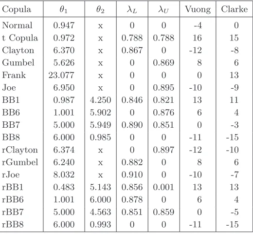
We also calculated locally best models on the system of 2-years’ intervals mentioned above. Development of their rating scores based both on Vuong and Clarke tests for all considered couples are presented in Figures 5, 6, 7. A clear local dominance of the Student class models is demonstrated.
Figure 6. Evolution of scoring based on Vuong (left) and Clarke (right) tests for couple bar & ml.
Figure 7. Evolution of scoring based on Vuong (left) and Clarke (right) tests for couple dj & ml.
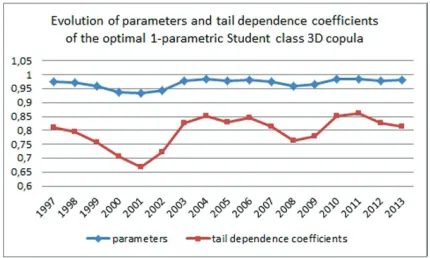
Figure 8 contains graphs of development of the parameters and tail depen-dence coefficients of the best Student local models.
Finally, Figure 9 contains comparable graphs of the development of the pa-rameters and tail dependence coefficients of the optimal one-parametric Student 3D models.
Figure 9. Evolution of parameters and tail dependence coefficients of the optimal 1-parametric Student class 3D copula.
5. Concluding remarks
We concluded that the returns of the considered bond indices have very high coefficients tail dependence and thus do not represent suitable components of well diversified portfolios. On the other hand, their optimal models are in the Student class with low degrees of freedom (only 2!) that implies high values of quantile functions, hence they could be good candidates for underlying assets of derivative instruments.
The results of our modeling are very impressive. The trends in development of the outcomes of the local models are surprisingly parallel. The values of pair-wise correlations between the considered inputs as well as of the calculated co-efficients of tail dependence of local optimal partial pairwise 2D copulas and one-parametric local 3D Student copulas exhibit extremely similar behavior.
REFERENCES
[1] BELGORODSKI, N.:Selecting Pair-Copula Families for Regular Vines with Application to the Multivariate Analysis of European Stock Market Indices.Diploma thesis, Technis-che Universitaet MuenTechnis-chen,http://mediatum.ub.tum.de/?id=1079284
[3] FERREIRA, M.:Nonparametric estimation of the Tail-dependence coefficient,REVSTAT
11(2013), 1–16.
[4] FRANSES, P. H.—DIJK, D.: Non-Linear Time Series Models in Empirical Finance.
Cambridge University Press, Cambridge, 2000.
[5] GENEST, C.—RIVEST, L.-P.:Statistical inference procedures for bivariate Archimedean copulas, J. Amer. Statist. Assoc.88(1993), no. 423, 1034–1043.
[6] GENEST, C.—R ´EMILLARD, B.—BEAUDOIN, D.: Goodness-of-fit tests for copulas: A review and a power study, Insur. Math. Econ.44(2009), 199–213.
[7] HOFERT, M.—KOJADINOVIC, I.—MAECHLER, M.—YAN, J.:Copula: Multivariate Dependence with Copulas. R package version 0.999-13, 2015.
http://CRAN.R-project.org/package=copula
[8] NELSEN, R. B.:An Introduction to Copulas(2nd ed.), in: Springer Ser. Stat., Springer--Verlag, New York, 2006.
[9] R CORE TEAM.:R: A language and environment for statistical computing, R Foundation for Statistical Computing, Vienna, Austria, 2015.https://www.R-project.org/ [10] SCHEPSMEIER, U. ET AL.:VineCopula: statistical inference of vine copulas, R package
version 1.6–1, 2015.http://CRAN.R-project.org/package=VineCopula
[11] SKLAR, A.:Fonctions de r´epartition a n dimensions et leurs marges, Publ. Inst. Statist. Univ. Paris8(1959), 229–231.
[12] VUONG, Q. H.:Ratio tests for model selection and non-nested hypotheses, Econometrica
57(1989), 307–333.
Received April 13, 2017 Jozef Komorn´ık
Faculty of Management Comenius University Odboj´arov 10 SK–831-04 Bratislava SLOVAKIA
E-mail: [email protected]
Magdal´ena Komorn´ıkov´a Tom´aˇs Bacig´al
Faculty of Civil Engineering STU Radlinsk´eho 11
SK–810-05 Bratislava SLOVAKIA
E-mail: [email protected] [email protected]
Cuong Nguyen Faculty of Commerce Lincoln University NZ Canterbury
NEW ZEALAND